In this short case study, we introduce the Portfolio Risk Parity tool. Risk parity is an investment management strategy that focuses on risk allocation. The main aim is to find such weights of assets that make up a portfolio to ensure an equal level of risk. The risk, in this case, is measured by 126-day volatility. The final portfolio is compared to a benchmark equally-weighted portfolio. Quantpedia Pro contains reports for three risk parity methodologies – Naive Risk Parity (inverse volatility weighted), Equal Risk Contribution and Maximum Diversification. Detailed info about all methodologies is available in the following article.
What does the typical report display? The report first shows the cumulative performance of the benchmark strategy, the performance table and the chart of the weights and volatility contribution. Secondly, it calculates the weights applying one of the three Risk Parity methodologies and displays the cumulative performance of the Risk Parity portfolio compared to the equally-weighted portfolio. Additionally, you can review the performance table of both portfolios and the charts of the weights, Volatility Contributions, Marginal Risk Contributions and Diversification Ratio of the Naïve Risk Parity portfolio.
Let’s look at how it actually works in practice. We use a portfolio containing four assets SPY (SPDR S&P 500 ETF), EFA (iShares MSCI EAFE ETF), GLD (SPDR Gold Trust) and IEF (iShares 7-10 Year Treasury Bond ETF) and our example shows Naive Risk Parity (inverse volatility weighted) method. Firstly, let’s take a look at the performance table of the two strategies.
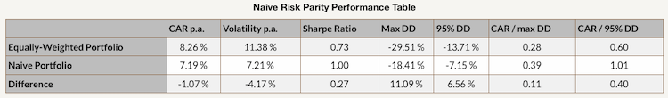
As we can see, the Naïve Risk Parity portfolios performance is lower compare to the equally-weighted portfolio. However, the volatility of the Naïve Risk Parity portfolio is significantly lower, resulting in a higher Sharpe ratio. Additionally, the CAR/max DD and CAR/95% DD are also higher, meaning the drawdowns are not as significant when applying Naïve Risk Parity.
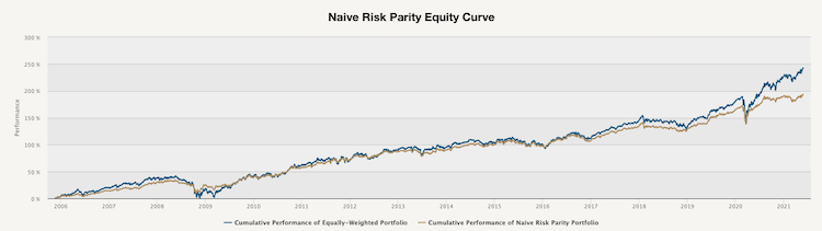
This chart shows how to performance evolved over time. As we can see, the cumulative performance of the Naïve Risk Parity portfolio is lower, however, as we already mentioned, the volatility and drawdowns are much less significant. The following figure shows the weights and risk contributions of the equally weighted portfolio.
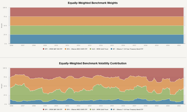
And now, let’s compare the weights and risk contributions of an equally-weighted portfolio and the Naïve Risk Parity portfolio.
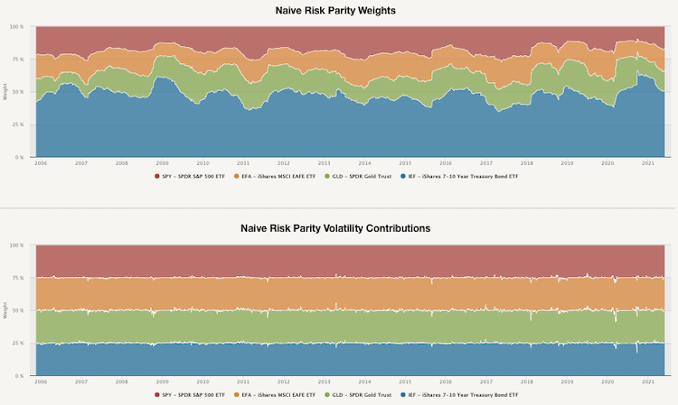
The top figure shows the weights of the assets in our portfolio. The bottom figure shows the volatility contribution of each asset. The volatility contribution of each ETF is nearly equal when using Naïve Risk Parity. Lastly, let’s look at marginal risk contribution and the diversification ratio.
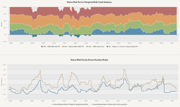
The top chart shows how the marginal risk contribution evolved over time. Marginal risk contribution is one step further than the volatility contribution. It is calculated similarly, but it takes to consideration the correlation between assets. To find each asset’s marginal contribution, take the cross-product of the weights vector and the covariance matrix divided by 126-day volatility of the portfolio. The bottom chart compares the diversification ratio of the Naïve Risk Parity portfolio and the equally-weighted portfolio. Portfolio’s diversification ratio is calculated as the ratio between weighted volatility of the assets and volatility of the whole portfolio. The higher the ratio, the more diversified the portfolio. As we can see, the diversification ratio of the Naïve Risk Parity portfolio is higher at almost every point in time.
Interested? Then subscribe to Quantpedia Pro and try how our analytics and reporting significantly saves time spent on quantitative research. Or check Quantpedia Explains if you would like to see more case studies.