Risk Parity Asset Allocation
This article is a primer into the methodology we use for the Portfolio Risk Parity report, which is a part of our Quantpedia Pro offering. We explain three risk parity methodologies – Naive Risk Parity (inverse volatility weighted), Equal Risk Contribution and Maximum Diversification. Quantpedia Pro allows the design of model risk parity portfolios built not just from the passive market factors (commodities, equities, fixed income, etc.) but also from systematic trading strategies and uploaded user’s equity curves.
Introduction
Risk parity is an investment management strategy that focuses on risk allocation. The main aim is to find weights of assets that ensure an equal level of risk, most frequently measured by volatility of the portfolio. To allocate the correct “risk parity” weight to an asset, we must understand its risk (and in some variations also return) characteristics. As the simplest benchmark, we use an equally weighted portfolio.
An equally weighted portfolio can be a great choice in many cases; however, when it comes to risk, it has one significant disadvantage. Imagine, we have an equally weighted portfolio consisting of ten assets, of which all but one are highly volatile. In this case, the one low volatile asset brings no diversification benefit. Additionally, the risk contribution of each of the nine highly volatile assets (such as stocks or commodities) is much larger than the risk contribution of the one low volatile asset (such as bonds).
We use simple historical 126-day volatility as a measure of risk. Marginal risk contribution of an asset is calculated as a product of marginal contribution and the weight of the asset divided by 126-day volatility of the portfolio. To find each asset’s marginal contribution, take the cross-product of the weights vector and the covariance matrix divided by 126-day volatility of the portfolio. Portfolio’s diversification ratio is calculated as the ratio between weighted volatility of the assets and volatility of the whole portfolio. The higher the ratio, the more diversified the portfolio. The data are sourced by the EOD Historical Data, also known as EODhd, a partner of this blog and provider of historical prices and fundamental financial data APIs.
Equally-Weighted Portfolio
The following figures show an equally weighted portfolio consisting of SPY (US equities), EFA (EAFE equities), GLD (Gold) and IEF (US 7-10y bonds) ETFs. The figure in the top left shows the weights of the ETFs. As the name suggests, each of the four ETFs has a quarter of the weight in the equally weighted portfolio. The top right figure shows the volatility contribution of each ETF in case of our benchmark equal weight allocation. The bottom left figure shows marginal risk contribution, and the figure in the bottom right shows the diversification ratio.
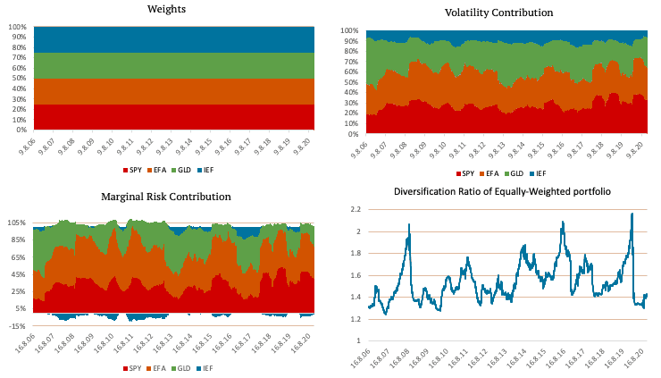
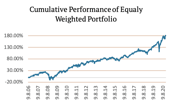
As you can see in the Volatility Contribution graph and the Marginal Risk Contribution graph, the diversification benefit of IEF (US 7-10y bonds) is minimal. Most of the portfolio’s risk is in the SPY (US equities) and EFA (EAFE equities) ETFs. The following figure shows the Cumulative Performance of Equally-Weighted Portfolio.
Naïve Risk Parity
In order to give a low volatile asset an equal opportunity to contribute to a portfolio, we can use naïve risk parity. Naïve risk parity or naïve risk weighting does not use equal weights. Instead, it uses the inverse risk approach. This approach gives lower weight to riskier assets and more significant weight to less risky assets. This method ensures that the risk contribution of each asset is the same.
Theoretically, naïve risk parity is based on the assumption that all the assets in the portfolio have a similar excess return per unit of risk; in other words, have similar Sharpe Ratios. However, the assets’ correlation cannot be determined with high confidence, i.e. it is omitted from the calculation.
There are multiple ways to measure the risk, i.e. input for the risk parity allocation. The most commonly used is volatility; however, variance, Value at Risk (VAR), Conditional Value at Risk (CVar), Conditional Drawdown at Risk (CDaR) or Maximum Daily Loss, and many more can also be used. In the case of normally distributed data, all the listed methods should agree on the optimal asset weights.
Calculating volatility is equal to calculating the standard deviation of daily returns. When the volatility is calculated, we assign the weights using the inverse risk approach:
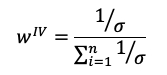
where sigma stands for the vector of asset volatilities.
The following figures show a portfolio consisting of SPY, EFA, GLD and IEF ETFs created using Naïve Risk Parity. The top left figure shows the weights of the ETFs. As you can see, the weights are no longer the same. IEF, an ETF consisting of US 7-10y bonds, has the greatest weight, because of its low volatility.
The top right figure shows the volatility contribution of each ETF. The volatility contribution of each ETF is nearly equal when using naïve risk parity. The bottom left figure shows marginal risk contribution, and the figure in the bottom right shows the comparison of diversification ratio of Equally-Weighted portfolio and Naïve Risk-Parity portfolio.

In the following table, we compare the risk metrics of Equally-Weighted portfolio and Naïve Risk-Parity portfolio.
|
|
14Y CAR |
14Y Volatility |
SR |
Max DD |
95% DD |
CAR/ |
CAR/ |
|
Equally-Weighted |
7.73% |
11.52% |
0.67 |
-29.58% |
-14.70% |
0.26 |
0.53 |
|
Naive Risk-Parity |
7.16% |
7.33% |
0.98 |
-19.04% |
-8.10% |
0.38 |
0.88 |
|
Difference |
-0.57% |
-4.19% |
0.31 |
10.54% |
6.60% |
0.11 |
0.36 |
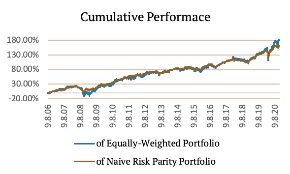
The following figure shows the Cumulative Performance of Naïve Risk-Parity Portfolio.
Equal Risk Contribution
Secondly, we will take a look at “true risk parity” also known as equal risk contribution (ERC). This method also tries to equalize the risk contribution of assets. If all the assets had a correlation equal to one, the equal risk contribution would assign the same weights as naïve risk parity. However, this method takes into consideration the historical correlations of the assets which is not equal to 1.
Imagine, we have a portfolio consisting of ten assets, of which all but one are mildly volatile. Additionally, the remaining one is highly volatile and has a negative correlation to the others. If we used naïve risk parity, the risk allocation would simply penalize the high volatility of the risky asset, and the low correlation of the risky asset would not bring any benefit. In this case, the equal risk contribution is more suitable than naïve risk parity, because it gives greater weight to the asset with low correlation.
To incorporate benefits from the correlation between assets, we use equal risk contribution. This method considers the objectives of the equal-weight and minimum variance portfolios. Research shows [ReSolve – PORTFOLIO OPTIMIZATION- A GENERAL FRAMEWORK FOR PORTFOLIO CHOICE] that the final portfolio will have volatility between that of the minimum variance portfolio and the equal-weight portfolio.
Finding the weights for the assets is not as easy as with naïve risk parity. The weights are calculated using the following convex optimization:
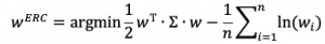
where capital Sigma is the covariance matrix.
The following figures show a portfolio consisting of SPY, EFA, GLD and IEF ETFs created using Equal Risk Contribution. The top left figure shows the weights of the ETFs. Once again, the weights are not the same. IEF, an ETF consisting of US 7-10y bonds, has the greatest weight, because of its low volatility and low correlation to the other ETFs.
The top right figure shows the volatility contribution of each ETF. The volatility contribution of each ETF is not entirely equal as with naïve risk parity. However, it is still relatively stable. Additionally, the bottom left figure shows that marginal risk contribution of all four ETFs is almost equal. The figure in the bottom right shows the comparison of diversification ratio of Equally-Weighted portfolio, Naïve Risk-Parity portfolio and Equal Risk Contribution portfolio.
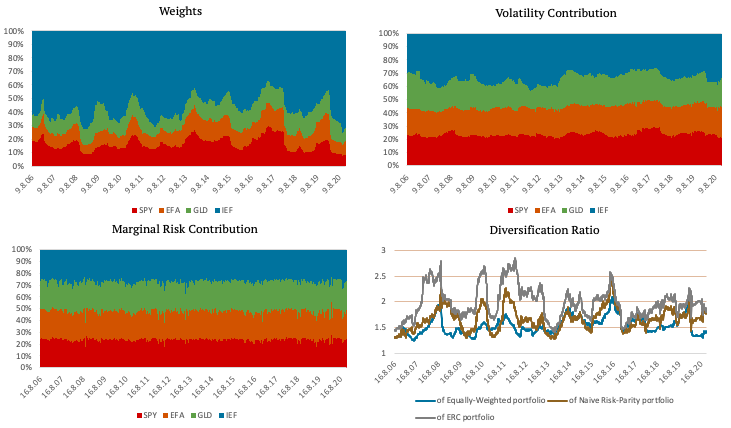
We can see that even though the weights are not stable at all, the Marginal Risk Contribution of each ETF is almost equal. The following table compares the risk metrics of Naïve Risk-Parity portfolio and ERC portfolio.
|
|
14Y CAR |
14Y Volatility |
SR |
Max DD |
95% DD |
CAR/ |
CAR/ |
|
Naive Risk-Parity |
7.16% |
7.33% |
0.98 |
-19.04% |
-8.10% |
0.38 |
0.88 |
|
ERC Portfolio |
6.93% |
6.12% |
1.13 |
-15.28% |
-6.01% |
0.45 |
1.15 |
|
Difference |
-0.23% |
-1.21% |
0.16 |
3.76% |
2.09% |
0.08 |
0.27 |
The following figure shows the Cumulative Performance of ERC Portfolio.

Maximum Diversification
Last but not least, let’s introduce the maximum diversification method. This method differs from CAPM and does not assume that returns are proportional to systematic risk. On the contrary, it proposes risk-efficient markets, where all returns of investments are proportionate to their total risk, measured by volatility. Thus, we can say that returns are proportional to volatility. Maximum Diversification optimization substitutes asset volatilities for returns in a maximum Sharpe ratio optimization, taking the following form:

where sigma denotes a vector of volatilities and capital Sigma denotes the covariance matrix.
The aim of this optimization is to maximize the ratio between the weighted average of the portfolio’s components’ volatility and the total portfolio volatility. Which is the same as maximizing the weighted average return if we assume the return and volatility are directly proportional.
If we had a portfolio of perfectly correlated assets, such a portfolio’s volatility would be equal to the weighted sum of its components’ volatilities. There would not be an opportunity for diversification. If the assets are not perfectly correlated, the weighted average volatility grows larger than the portfolio volatility in proportion to the available diversification.
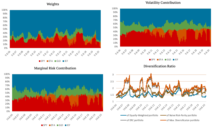
The following figures show a portfolio consisting of SPY, EFA, GLD and IEF ETFs created using Maximum Diversification. The top left figure shows the weights of the ETFs. Once again, IEF, an ETF consisting of US 7-10y bonds, has the greatest weight.
The top right figure shows the volatility contribution of each ETF, and the bottom left figure shows that marginal risk contribution of all four ETFs. The figure in the bottom right shows the comparison of diversification ratio of Equally-Weighted portfolio, Naïve Risk-Parity portfolio, Equal Risk Contribution portfolio and Maximum Diversification portfolio.
Additionally, we present a table that compares the risk metrics of ERC portfolio and Maximum Diversification portfolio.
|
|
14Y CAR |
14Y Volatility |
SR |
Max DD |
95% DD |
CAR/ |
CAR/ |
|
ERC Portfolio |
6.93% |
6.12% |
1.13 |
-15.28% |
-6.01% |
0.45 |
1.15 |
|
Maximum Diversification |
6.78% |
5.54% |
1.23 |
-12.99% |
-5.22% |
0.52 |
1.30 |
|
Difference |
-0.15% |
-0.58% |
0.09 |
2.29% |
0.79% |
0.07 |
0.15 |
The following figure shows the Cumulative Performance of Maximum Diversification Portfolio.

Lastly, we can take a look at the following table. The table shows all the risk metrics we used for all of the abovementioned methods. Each strategy is rebalanced on a weekly basis, plus there is one “skip-day” between the calculation of the weights and rebalancing.
|
|
14Y CAR |
14Y |
SR |
Max DD |
95% DD |
CAR/ |
CAR/ |
|
Equally |
7.73% |
11.52% |
0.67 |
-29.58% |
-14.70% |
0.26 |
0.53 |
|
Naive |
7.16% |
7.33% |
0.98 |
-19.04% |
-8.10% |
0.38 |
0.88 |
|
ERC |
6.93% |
6.12% |
1.13 |
-15.28% |
-6.01% |
0.45 |
1.15 |
|
Maximum |
6.78% |
5.54% |
1.23 |
-12.99% |
-5.22% |
0.52 |
1.30 |
Author:
Daniela Hanicova, Quant Analyst, Quantpedia
Are you looking for more strategies to read about? Sign up for our newsletter or visit our Blog or Screener.
Do you want to learn more about Quantpedia Premium service? Check how Quantpedia works, our mission and Premium pricing offer.
Do you want to learn more about Quantpedia Pro service? Check its description, watch videos, review reporting capabilities and visit our pricing offer.
Do you want algorithmic access to the full Quantpedia database via the API? Subscribe to Quantpedia Pro, ask for an API key, and explore the in/out-of-sample statistics, source academic papers, and code snippets — ideal for quantitative research, systematic trading workflows, and AI model training.
Are you looking for historical data or backtesting platforms? Check our list of Algo Trading Discounts.
Or follow us on:
Facebook Group, Facebook Page, Telegram, Twitter, Linkedin, Medium or Youtube
Share onLinkedInTwitterFacebookRefer to a friend


