100-Years of the United States Dollar Factor
Finding high-quality data with a long history can be challenging. We have already examined How To Extend Historical Daily Bond Data To 100 years, How To Extend Daily Commodities Data To 100 years, and How To Build a Multi-Asset Trend-Following Strategy With a 100-year Daily History. Following the theme of our previous articles, we decided to extend historical data of a new factor, the Dollar Factor. This article explains how to combine multiple data sources to create a 100-year daily data history for the Dollar Factor, introduces data sources, and explains the methodology.
Edit: The article was edited on the 28th of September. We fixed calculation issues in the estimation of the USD exchange rate in the period 1926-1971.
What is the Dollar Factor?
The Dollar Factor measures the value of the United States Dollar (USD) relative to its most important trading partners’ currencies. Currently, the six foreign currencies are used for the calculation of the US Dollar Index (DXY): Euro (EUR), Japanese Yen (JPY), Pound Sterling (GPB), Canadian Dollar (CAD), Swedish Krona (SEK), and Swiss Franc (CHF). The Dollar Index goes up as the dollar strengthens compared to the aforementioned currencies. To some extent, it reflects the US economy relative to the rest of the world. However, the historical data of DXY cover only the time range from 1971 until the present. Therefore, we have collected multiple data from 1926 to help us extend historical data for the Dollar Factor.
How to build a 100-year daily history of the Dollar Factor?
To create the 100-year history of the Dollar Factor we’ve combined multiple data sources:
1926-1953
The data from 1926 to 1953 were obtained from riksbank.se. Firstly, we collected monthly exchange rates of the Swedish krona (SEK) to several historically relevant currencies: US Dollar (USD), Deutschmark (DEM), Pound Sterling (GBP), French Franc (FRF), Belgian Franc (BEF), Swiss Franc (CHF), Dutch Guilder (NLG), Danish Krone (DKK), Norwegian Krone (NKK), and Italian Lira (ITL). Secondly, to determine the exchange rate of USD to other currencies (denoted as XYZ), we applied the basic formula:

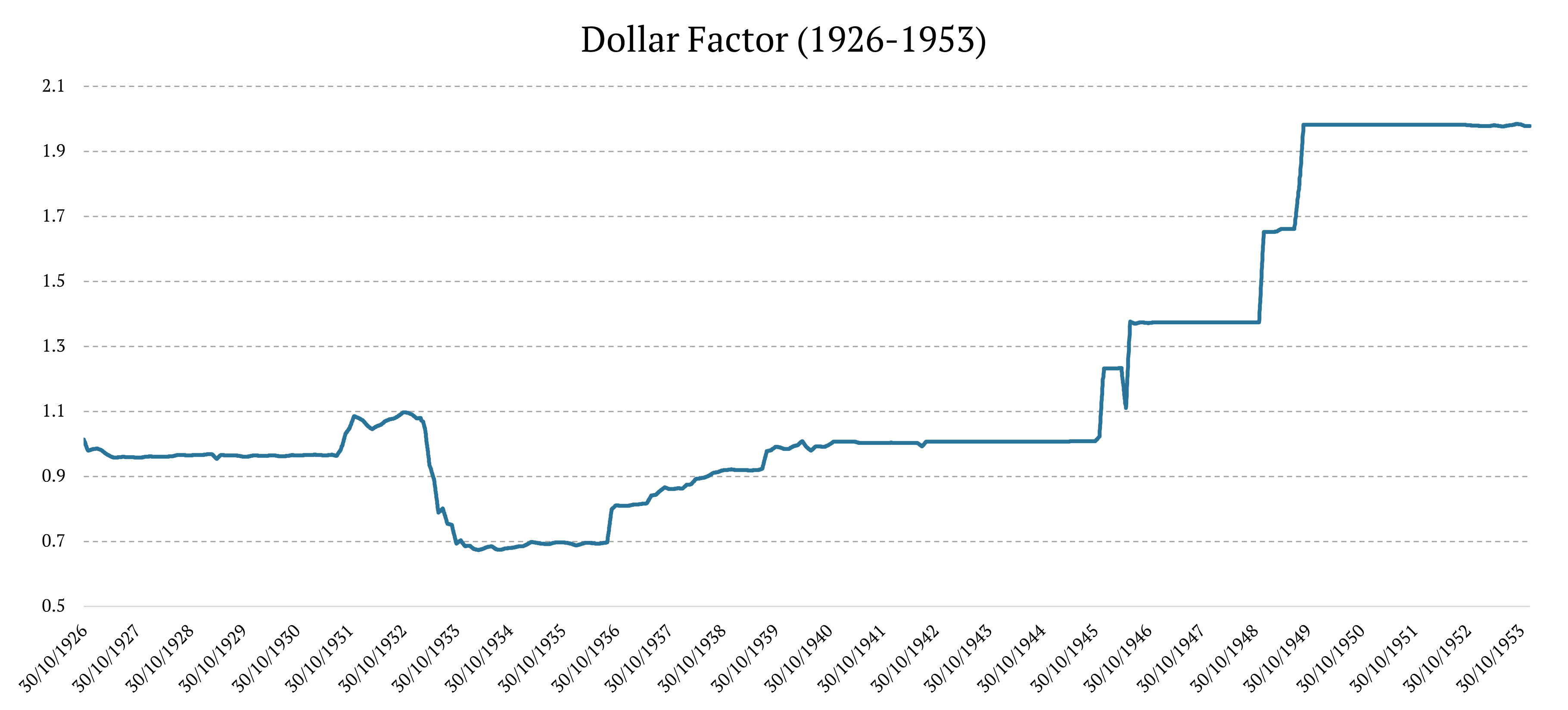
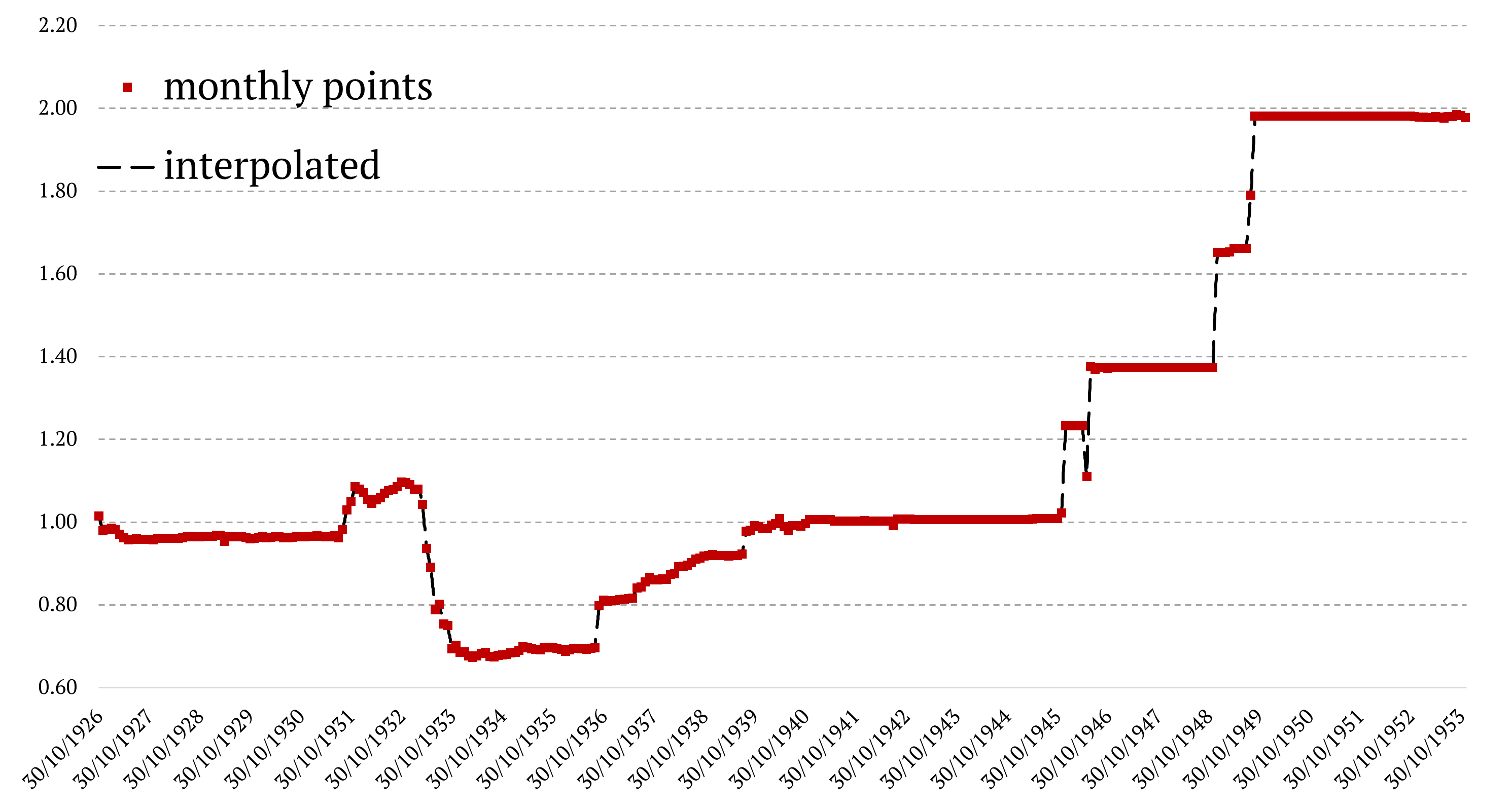
As we obtained the monthly exchange rates, we calculated monthly performances for every pair USD/XYZ. Finally, using GDP from Wikipedia’s List of regions by past GDP for Europe: 1830–1938 (Bairoch) as weights, we calculated the index using the 1925 GDP value for the time interval 1926-1937, and the 1938 GDP value for the time interval 1938-1953. Unfortunately, our data are at a monthly frequency only. Therefore, we describe how to transform them into daily data below.
As we can see on the graph, significant changes marked the 1930s and 1940s. In 1933 US Dollar rapidly deteriorated compared to the Deutschmark, Pound Sterling, and French Franc. What was the reason for these changes?
In 1933, the United States suspended the gold standard, an imbalance between USD currency and those of the gold bloc grew (for example, France). This imbalance caused the US Dollar devaluation, raising import prices and lowering export prices in the United States. Finally, the Tripartite Agreement stabilized exchange rates and ended the currency war from 1931 to 1936.
The rise of the USD in the late 1940s was caused by the significant strength of the US economy compared to its usual peers (European countries like France, the UK, Germany, Benelux countries, and northern Europe) that were weakened after WW2. The United States emerged as a clear winner of the war, and a series of devaluations against the USD followed in the late 1940s.
1953-1971
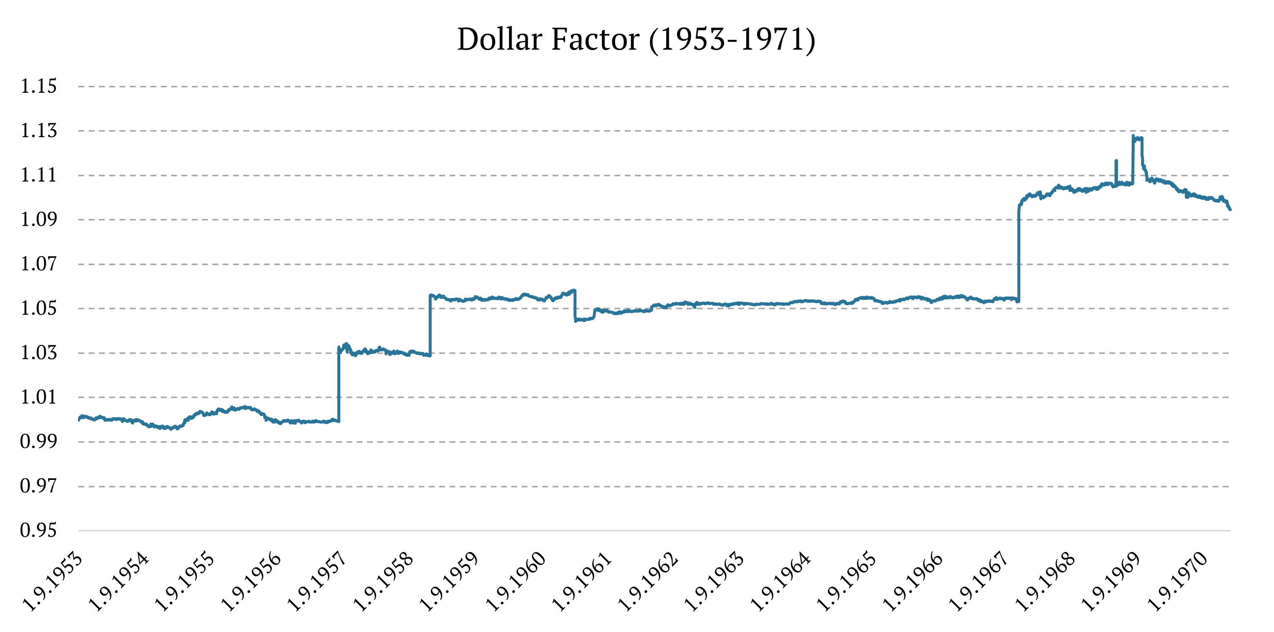
The data from 1953 to 1971 were obtained from bis.org. For the second period, we collected the daily exchange rates of US Dollar against several currencies: Belgian Franc (BEF), Canadian Dollar (CAD), Swiss Franc (CHF), Deutschmark (DEM), Danish Krone (DKK), French Franc (FRF), Pound Sterling (GBP), Italian Lira (ITL), Dutch Guilder (NLG), Norwegian Krone (NOK), and Swedish Krona (SEK). To calculate the Dollar Factor, we had to calculate daily performances and similar to the first period, we used GDP as weights to calculate the index. However, for this period, we used the values from List of regions by past GDP for World: 1–2008 (Maddison) for the year 1950.
1971-2022
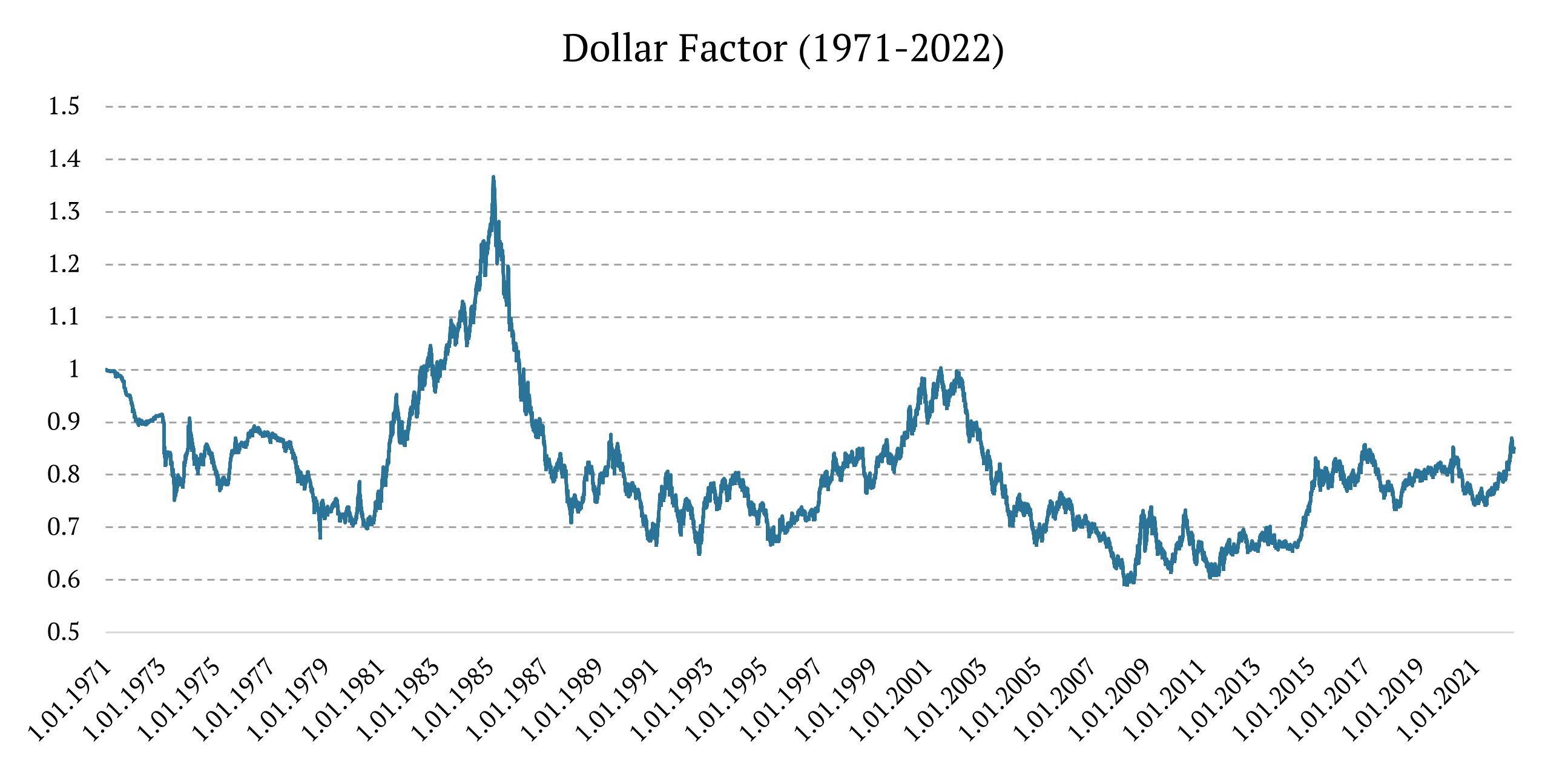
Lastly, the data from 1971 to 2022 were obtained from Wikipedia’s U.S. Dollar Index. So, from 1971 to the present, we have followed up with the daily data of the US Dollar Index (DXY).
Transforming Monthly Data into Daily Data
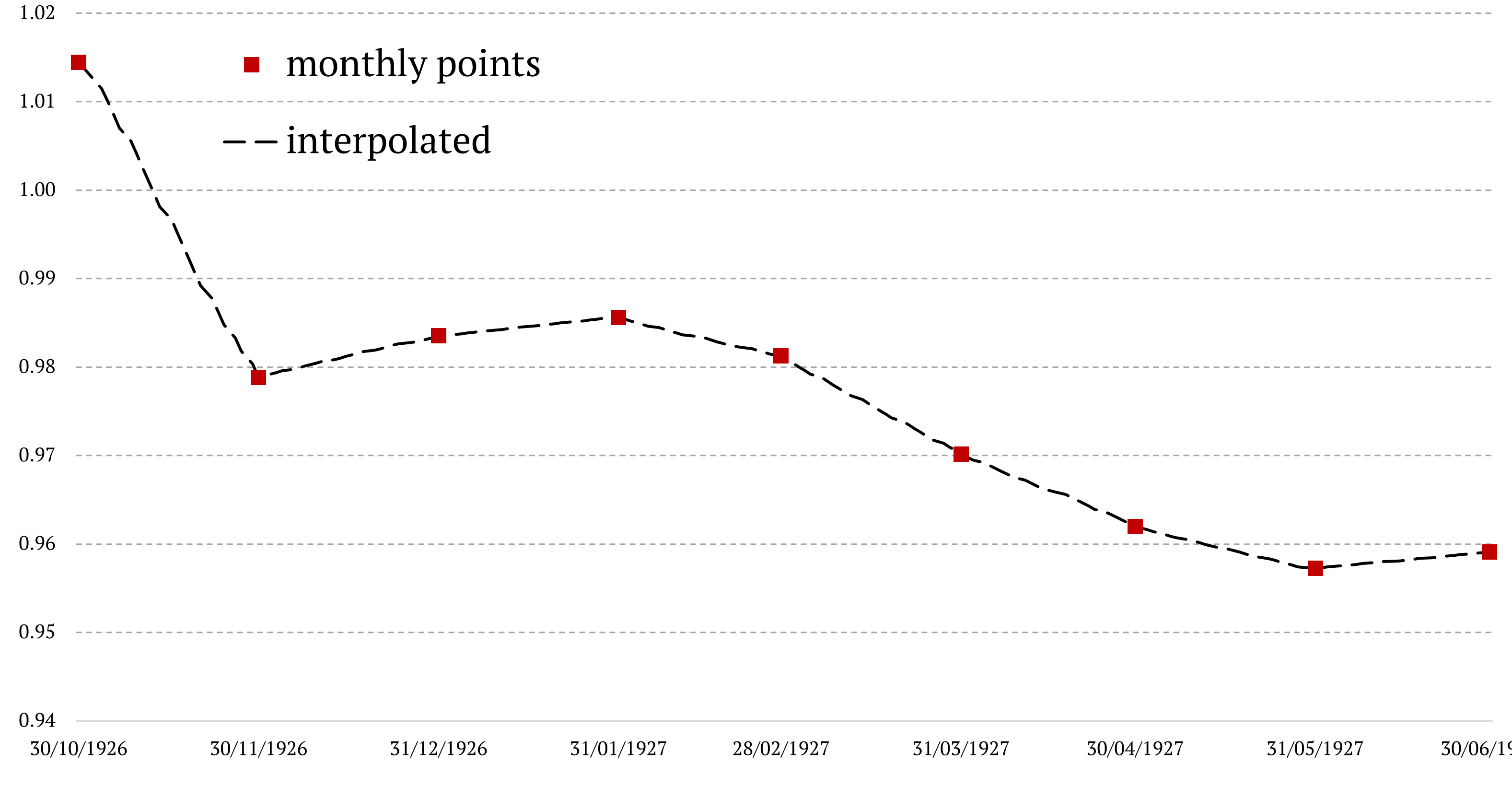
As we have already mentioned, it is necessary to transform the monthly data from the first sub-period (1926-1953) into daily data. On the other hand, the data from the last two sub-periods (1953-2022) were on a daily frequency, so there is no need to modify them. Unfortunately, there is no daily proxy to estimate the daily volatility for the first period. For that reason, we applied simple linear interpolation, similar to the one we used in Extending Historical Daily Bond Data to 100 Years. In the first step, we calculated the cumulative difference between the two data points every month and got the daily interest. Subsequently, we cumulated the respective interests each day. Yet, there is a disadvantage of the linear interpolation – the resulting curve has zero intra-month volatility.
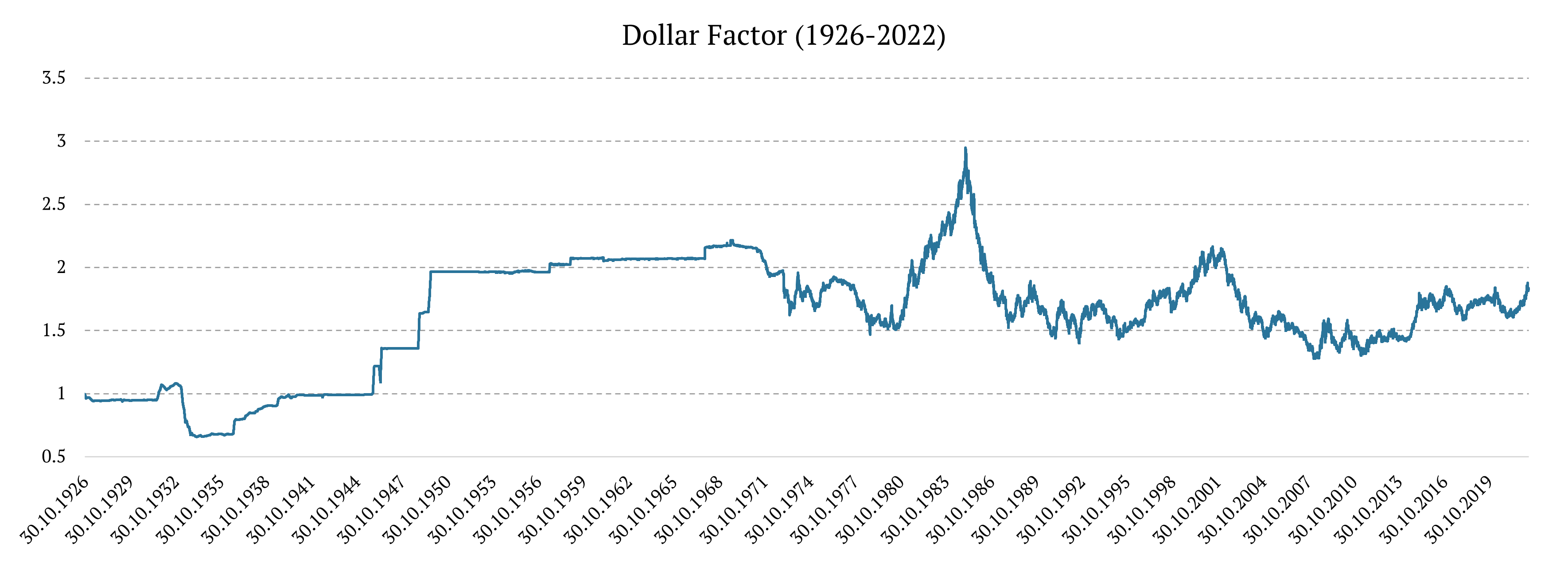
Combining Various Data Sources
Finally, we combined the data series from three different periods into one time series.
At the close of the article, we would like to mention that the history of the exchange rate is not sufficient if we want to analyze the behavior of the currencies. In each currency, the central bank interest rates history is also essential for investors, economists, and even everyday savers. This historical data provides insight into economic cycles, helping predict future movements and understand the long-term effects of monetary policies. For example, in the wake of the 2008 financial crisis, many central banks slashed interest rates to near-zero levels to stimulate their economies, and only in recent years have some begun raising them again.
If you’re interested in learning more or tracking how interest rates have evolved over time, you can check our article that explains how to combine multiple data sources to create a 100-year daily data history for US 10-year bonds, or you can review this central bank interest rates history table that offers a comprehensive view of the rates set by major global banks.
Authors:
Juliana Javorska, Quant Analyst, Quantpedia
Daniela Hanicova, Quant Analyst, Quantpedia
Are you looking for more strategies to read about? Sign up for our newsletter or visit our Blog or Screener.
Do you want to learn more about Quantpedia Premium service? Check how Quantpedia works, our mission and Premium pricing offer.
Do you want to learn more about Quantpedia Pro service? Check its description, watch videos, review reporting capabilities and visit our pricing offer.
Are you looking for historical data or backtesting platforms? Check our list of Algo Trading Discounts.
Would you like free access to our services? Then, open an account with Lightspeed and enjoy one year of Quantpedia Premium at no cost.
Or follow us on:
Facebook Group, Facebook Page, Twitter, Linkedin, Medium or Youtube
Share onLinkedInTwitterFacebookRefer to a friend