An Introduction to Volatility Targeting
One of the most popular reports in the Portfolio Analysis section of our Quantpedia Pro tool is “Volatility Targeting”. In this article, we will explain some theory behind this portfolio management method. And then, we will go more in-depth, pick several examples and explain some common volatility targeting variants.
What is volatility and how to target it?
Volatility is the most common risk metric of a stock. The main aim of the volatility targeting technique is to manage the portfolio’s exposure in such a way that the volatility of a portfolio is as close to the target value as possible. In other words, to ensure that the amount of dollar risk remains the same. To do this, the portfolio manager has to increase or decrease the amount of leverage, depending on the volatility.
If the volatility goes up, he/she has to scale down the portfolio. On the other hand, if the volatility goes down, he/she should take more leverage. Volatility target is the level of annual volatility to which the portfolio is adjusted.
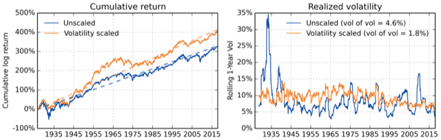
As is illustrated in the figure below, smoothing of the volatility is an effect of volatility targeting. Even though this may not necessarily help the performance, smooth volatility is easier to predict. The following figure shows cumulative returns and realized volatility for all US Equities. We can see that the volatility of volatility is significantly reduced by volatility scaling. Pictures 1. to 3. are from the research paper “The Impact of Volatility Targeting“, written by Harvey, Hoyle, Korgaonkar, Rattray, Sargaison and Van Hemert, which we really recommend to anybody interested in the subject of volatility scaling/targeting.
Pic.1 – Cumulative returns and realized volatility for all US Equities. Volatility-scaling is done using exponentially-decaying weights with a half-life of 20 days.
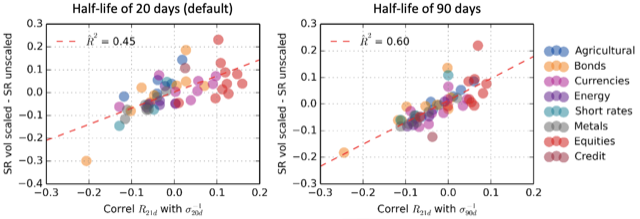
Numerous researches argue that Sharpe Ratios increase under volatility targeting. Specifically, for the so-called “risk assets” such as equity and credit, the Sharpe Ratio increases with the accuracy of volatility predictions that are used to implement the strategy. However, for bonds, currencies, commodities, and other assets is the impact on Sharpe ratio negligible. The change of Sharpe Ratios in various assets is illustrated in figures below.
Pic.2 – Improvement in SR when volatility scaling vs correlation (past returns, 1/vol) for various assets.
Methods of Volatility Targeting
There are multiple techniques of volatility targeting. The simplest one is portfolio volatility targeting. It is based on adjusting the level of exposure of the entire portfolio to target a constant level of volatility. It ignores the differences between the volatilities of assets inside the portfolio.
Dynamic Volatility Scaling
Portfolio volatility targeting can be upgraded by calculating the volatility of each instrument alone using long term data, plus using respective long-term correlation estimates to assess the degree to which they trade as a group. This technique is called dynamic volatility scaling. The portfolio manager is then able to reduce the exposure of each instrument as its volatility increases or raise the exposure as volatility falls.
Assuming the historically derived risk estimate provides an indication of the future risk, one may expect each instrument to have a more stable standalone risk contribution over time. Stable risk contribution of each asset is at the heart of this technique. As the next step, one may then apply portfolio volatility targeting. As the correlation between the instruments and asset classes goes up, portfolio manager reduces the overall exposure, and as it falls, the portfolio manager increases the exposure. The standalone risk allocations are scaled up and down to target a more stable broad risk exposure.
The only disadvantage of these techniques is the delayed reaction. However, there is also a danger in reacting too fast. An example of that can be a situation where markets mean revert. Reducing positions too fast could lead to losses on the downside plus additional trading costs as the measure will quickly revert to more normal levels.
Volatility Switching
Volatility switching solves this problem by introducing a faster measure of volatility. The faster measure is not implemented unless market conditions are going through substantial material changes, and it is necessary to de-risk the portfolio instantly.
Adding a Momentum Filter
The next technique covers adding a momentum filter. It aims for limiting losses even further by reducing risk levels in unfavorable markets. This technique depends on the extra observation of persistence in market returns. In the case, the asset prices start to fall, they have historically been slightly more likely to continue to fall than to recover. Under this scenario, we prefer to own less of markets that are falling. On the other hand, if the prices start to rise, they have historically been slightly more prone to rise even more. That means, we prefer to increase our allocation to these assets.
Volatility Targeting Step By Step
To summarize: the volatility scaling outlined above tends to reduce exposure when markets are dropping (because of the negative correlation between volatility and price returns). This reduction aims at keeping the constant level of risk. The momentum filter goes one step further and reduces exposures to deliver under target risk as long as prices are dropping. This might result in the strategy missing out on a few positive returns when markets switch from a negative trend to the positive one or vice versa. Yet, research agrees that it is worth missing on these turning points and reducing exposure to falling markets rather than sitting through the turbulence.
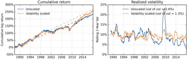
After scaling volatility, the performance of classical 60-40 equity-bond balanced portfolio slightly improves as is illustrated in the figure below. More importantly, the volatility is much smoother and easier to predict. Additionally, the volatility of volatility is significantly reduced.
Pic. 3. – Cumulative returns and realized volatility for 60-40 equity-bond balanced portfolio. Volatility-scaling (at both the asset and portfolio level) is done using exponentially-decaying weights with a half-life of 20 days.
Computational Models
We distinguish among two main types of volatility. The first one is the historical volatility, which is based on historical data. The second one is implied volatility. The assumption of historical volatility is that by knowing the past, we are able to predict the future. On the flip side, implied volatility solves for the volatility implied by present market prices.
Three most basic and widely used models for historical volatility are the following: Simple, Exponentially Weighted Moving Average (EWMA) and Generalized Auto-Regressive Conditional Heteroskedasticity (GARCH). To calculate these, one must follow a number of steps. The first step is to calculate a series of periodic returns, usually daily returns. Next step is to apply a weighting scheme, which is different for each type of volatility.
Simple Volatility
In calculations of simple volatility, the periodic returns are weighted equally, meaning that simple volatility is equal to the square root of the variance, which equals the arithmetic average of the squared returns. For example, let’s imagine we have daily returns for the last 30 days, then the weight for each return is 1/30. The most significant disadvantage of this approach is that recent returns have the same impact on the calculated level of volatility as returns from the past.
Equally-Weighted Moving Average
The EWMA method solves this by giving greater weight to more recent returns and smaller weight to past returns. The smoothing parameter lambda, which has to be less than one, is introduced in this method. The closer lambda is to one, the slower the decay in the series and the more data points we have in the series. On the other hand, the smaller the lambda is, the faster the decay in the series and the fewer data points are relevant. Under that requirement, rather than using equal weights, each squared return is weighted by a multiplier.
Generalized AutoRegressive Conditional Heteroskedasticity
Last, but not least is the GARCH method. As the name suggests, this method is Auto-Regressive and assumes conditional heteroskedasticity. This is especially useful because volatility tends to vary in time and is dependent on past variance, making a homoscedastic model suboptimal. GARCH process depends on past squared returns and past variances to model current variance. It is recommended to use this model if there are repeating periods of unexplained high volatility.
Examples of Volatility Targeting
Simple Volatility Targeting
The first example we explain in more detail is simple volatility targeting. The portfolio we analyze was created by combining two ETFs, specifically 60% of SPY and 40% of IEF. We chose this as our benchmark portfolio because of its popularity and diversification. Additionally, this portfolio can be classified as medium risk, which makes it a great candidate for volatility targeting.
In the first step, we estimate the volatility of our portfolio as the 20-day standard deviation of daily returns. Then a target is set. We decided to set an average of past volatility calculated in step 1 (expanding window from the start of the sample) as our target. After that, we calculate leverage as target volatility divided by the actual 20-day volatility; however, the maximal leverage we use is capped at two. Finally, we calculate the performance of the volatility targeted portfolio at day t as leverage, calculated from data till day t-2, multiplied by the daily performance at day t to avoid any look-ahead bias. The volatility targeted portfolio is rebalanced weekly.
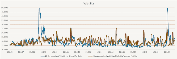
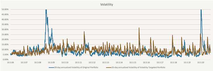
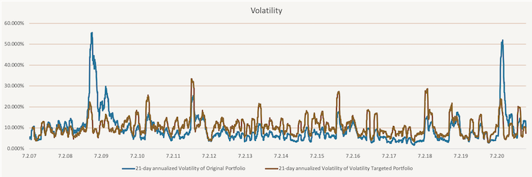
The figure below shows how the volatility of the original portfolio and volatility targeted portfolio changes in time. The main advantage of volatility targeted portfolio is that during the times of heightened volatility, the volatility of the targeted portfolio does not rise as much.
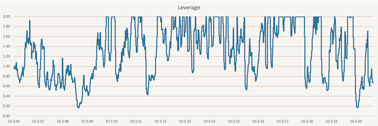
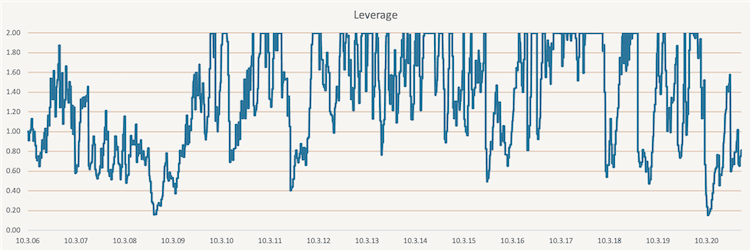
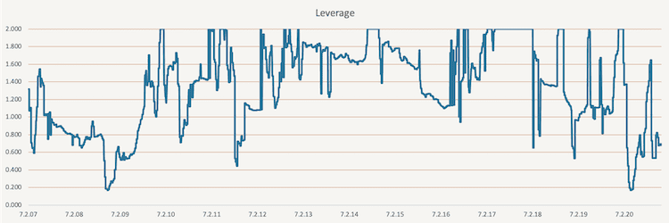
Additionally, to make this more realistic, we use 1-Month London Interbank Offered Rate (1-M LIBOR) as our cash rate. If the leverage is below one, meaning less than 100% of the portfolio is invested, we multiply the difference by the 1-M LIBOR and add the return to the volatility targeted portfolio. On the other hand, if the leverage is above one, meaning more than 100% of the portfolio is invested, we multiply the percentage above 100% by the 1-M LIBOR and subtract the return from the volatility targeted portfolio. The change of the leverage in time is illustrated in the figure below.
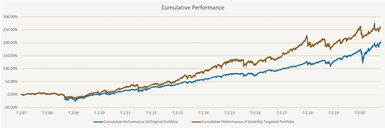
To compare the original portfolio and the volatility targeted portfolio, we calculated the performance metrics of both. As you can see in the table below, the 14-year annualized volatility of the original portfolio is above 11%; however, for the volatility targeted portfolio it stays at 10.59%. Additionally, while the 14-year annualized cumulative performance of the volatility targeted portfolio is above 10.7%, for the original portfolio it remains just under 9%. All return-to-risk ratios improved thanks to volatility targeting.
|
|
14Y CAR |
14Y Volatility |
SR |
Max DD |
95% DD |
CAR/ |
CAR/ |
|
Original Portfolio |
8.86% |
11.27% |
0.79 |
-31.39% |
-17.40% |
0.28 |
0.51 |
|
Volatility Targeted |
10.76% |
10.59% |
1.02 |
-19.48% |
-11.27% |
0.55 |
0.95 |
|
Difference |
1.90% |
-0.68% |
0.23 |
11.92% |
6.12% |
0.27 |
0.45 |
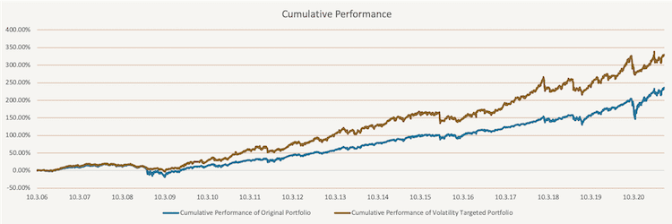
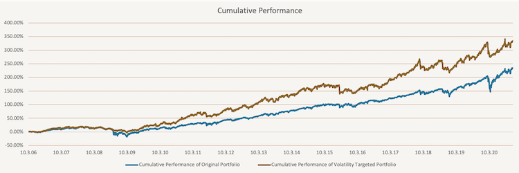
In this figure, we illustrate the performance of the benchmark portfolio and the volatility targeted portfolio since March 2006 till November 2020. It is apparent that the targeted portfolio has better performance from the start.
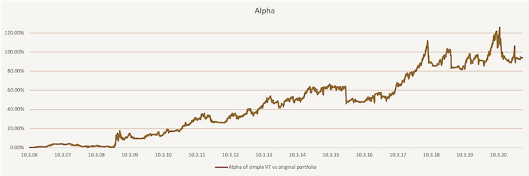
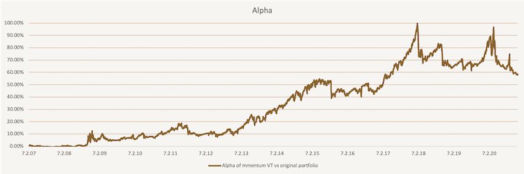
The figure below shows the Alpha of the simple volatility targeted portfolio against the original portfolio consisting of 60% of SPY and 40% if IEF.
EWMA Volatility Targeting
The second approach we take is using the Exponentially Weighted Moving Average (EWMA) volatility targeting. The main difference between this approach and simple volatility targeting is that simple volatility targeting gives equal weights to all returns. On the other hand, EWMA volatility targeting gives higher weight to the most recent return and smaller weight to the most distant return.
The figure below shows how the volatility of the original portfolio and volatility targeted portfolio changes in time. Similarly, to simple volatility targeting, the volatility of the volatility targeted portfolio is lower during the times of heightened volatility compared to the original portfolio.
To calculate the EWMA volatility of the original portfolio, we use the following formula:

Where ![]() is daily return, n=20 is the number of days and
is daily return, n=20 is the number of days and ![]() . Secondly, we set the target and calculate the leverage. We use the same method as we used in simple volatility targeting. The target is equal to the expanding window average of historical 20-day volatility, and leverage is calculated as target volatility divided by the actual 20-day volatility; however, the maximal leverage we use is two. Additionally, we use 1-Month London Interbank Offered Rate (1-M LIBOR) as our cash rate the same way as we did in simple volatility targeting. Finally, we calculate the performance of the volatility targeted portfolio at day t as leverage, calculated from data till day t-2, multiplied by the daily performance at day t. The volatility targeted portfolio is rebalanced weekly. The change of the leverage in time is illustrated in the figure below.
. Secondly, we set the target and calculate the leverage. We use the same method as we used in simple volatility targeting. The target is equal to the expanding window average of historical 20-day volatility, and leverage is calculated as target volatility divided by the actual 20-day volatility; however, the maximal leverage we use is two. Additionally, we use 1-Month London Interbank Offered Rate (1-M LIBOR) as our cash rate the same way as we did in simple volatility targeting. Finally, we calculate the performance of the volatility targeted portfolio at day t as leverage, calculated from data till day t-2, multiplied by the daily performance at day t. The volatility targeted portfolio is rebalanced weekly. The change of the leverage in time is illustrated in the figure below.
To compare the original portfolio and the volatility targeted portfolio, we again calculated return and risk metrics for both. As you can see in the table below, the 14-year annualized volatility of the original portfolio is almost 10%; however, for the volatility targeted portfolio it is just 8.09%. Additionally, while the 14-year annualized cumulative performance of the volatility targeted portfolio is above 10.8%, for the original portfolio it is just under 9%. Once again, all return-to-risk ratios clearly improved.
|
|
14Y CAR |
14Y Volatility |
SR |
Max DD |
95% DD |
CAR/ |
CAR/ |
|
Original Portfolio |
8.86% |
9.83% |
0.90 |
-31.39% |
-17.40% |
0.28 |
0.51 |
|
Volatility Targeted |
10.85% |
8.09% |
1.34 |
-18.92% |
-11.61% |
0.57 |
0.93 |
|
Difference |
1.99% |
-1.74% |
0.44 |
12.47% |
5.78% |
0.29 |
0.42 |
When we compare the performance of simple volatility targeted portfolio and EWMA volatility targeted portfolio, we can see that EWMA improves the performance even a bit further. This is the consequence of the weights used in the calculations. While simple volatility targeting uses equal weights, EWMA gives greater weights to the more recent data. In the figure below the performance of the benchmark portfolio and the EWMA volatility targeted portfolio are displayed since March 2006 till November 2020. Again, it is apparent that the targeted portfolio has better performance from the start.
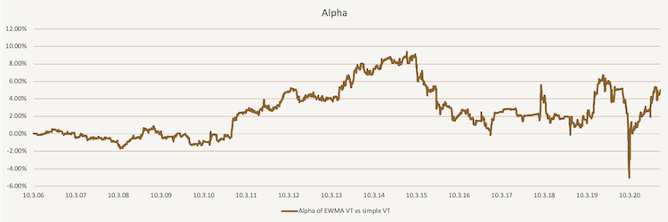
The figure below shows the Alpha of the EWMA volatility targeted portfolio against the simple volatility targeted portfolio.
Tactical Volatility Targeting
Instead of targeting volatility for the entire time, one may decide to do so only opportunistically. This gives way to another approach of volatility targeting we call tactical volatility targeting (or conditional volatility targeting). We examined several methods of conditional volatility targeting and for the sake of brevity decided to present one of them.
In the figure below, we show how the volatility of the original portfolio and tactically volatility targeted portfolio changes in time. Once again, the volatility of the targeted portfolio is less volatile.
This conditional method is based on a simple idea of momentum. Firstly, we create three simple volatility targeted portfolios, the same way we did in the first method, with different horizons. The horizons we picked are 21 days, 63 days and 252 days. Secondly, we calculate the 6-month performance of each of these portfolios. Lastly, once a week, we pick the portfolio with the best 6-month performance as our new volatility targeted portfolio. The leverage applied in the targeted portfolio is presented in the following figure. Once again, the maximal leverage is capped at two.
The calculated return and risk metrics for the original portfolio, and the volatility targeted portfolio are listed in the table below. As you can see, the 14-year annualized volatility did not change as much in this scenario. However, the 14-year annualized cumulative performance improved from 8.64% in the original portfolio to 10.21% in the volatility targeted portfolio.
|
|
14Y CAR |
14Y Volatility |
SR |
Max DD |
95% DD |
CAR/ |
CAR/ |
|
Original Portfolio |
8.64% |
11.52% |
0.75 |
-31.39% |
-17.87% |
0.28 |
0.48 |
|
Volatility Targeted |
10.07% |
11.43% |
0.88 |
-21.35% |
-13.33% |
0.47 |
0.76 |
|
Difference |
1.43% |
-0.10% |
0.13 |
10.05% |
4.54% |
0.20 |
0.27 |
Overall, the momentum-based tactical volatility targeting did not show significant improvement compared to the simple volatility targeting. However, the method still smoothed the volatility curve significantly and increased performance. In conclusion, this method (or other conditional ones) may be more effective than simple volatility targeting, but must be used on the right portfolio (ideally, one which is more trending). The following figure shows the improvement this method has on the performance of the 60% of SPY and 40% of IEF portfolio.
The figure below shows the Alpha of the momentum-based tactical volatility targeted portfolio against the original portfolio consisting of 60% of SPY and 40% if IEF.
All of the volatility targeting methods mentioned above can be reviewed and tested on a custom model portfolio assembled from any combination of passive market factors and/or systematic trading strategies available in the Quantpedia Pro. And it’s just one of the many features that may help you to speed up your quant research process.
Author:
Daniela Hanicova, Quant Analyst, Quantpedia
Are you looking for more strategies to read about? Sign up for our newsletter or visit our Blog or Screener.
Do you want to learn more about Quantpedia Premium service? Check how Quantpedia works, our mission and Premium pricing offer.
Do you want to learn more about Quantpedia Pro service? Check its description, watch videos, review reporting capabilities and visit our pricing offer.
Do you want algorithmic access to the full Quantpedia database via the API? Subscribe to Quantpedia Pro, ask for an API key, and explore the in/out-of-sample statistics, source academic papers, and code snippets — ideal for quantitative research, systematic trading workflows, and AI model training.
Are you looking for historical data or backtesting platforms? Check our list of Algo Trading Discounts.
Or follow us on:
Facebook Group, Facebook Page, Telegram, Twitter, Linkedin, Medium or Youtube
Share onLinkedInTwitterFacebookRefer to a friend


