Extending Historical Daily Bond Data to 100 Years
Introduction
Finding a good data source with quality data and long history is one of the greatest challenges in quantitative trading. There definitely are some data sources with very long histories. However, they tend to be on the more expensive side. On the other hand, cheap or free data usually lacks quality and/or has shorter time frames.
This article explains how to combine multiple data sources to create a 100-year daily data history for US 10-year bonds. Having a 100-year history of daily data can be very beneficial to understanding the market patterns and analyzing history and extending backtests to arrive at a new source of out-of-sample data.
Furthermore, suppose you want to examine how your portfolio would have performed during various historical events or to backtest a strategy during multiple market phases. In that case, the long history provides more opportunities. Besides, investors are always on the run to better understand the market. So, having substantial knowledge of history is crucial.
Underlying data and data sources
To create the 100-year history of the US 10-year bonds we’ve combined multiple data sources:
1926 – 1962: Monthly US 10-Year Bond Yields
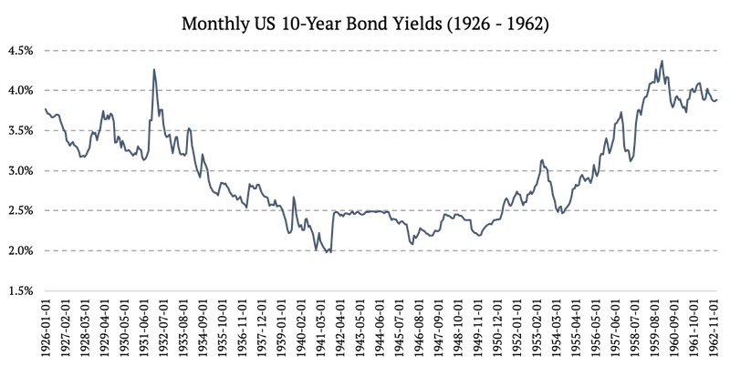
Source: https://fred.stlouisfed.org/series/LTGOVTBD
1962 – 2002: Daily US 10-Year Bond Yields
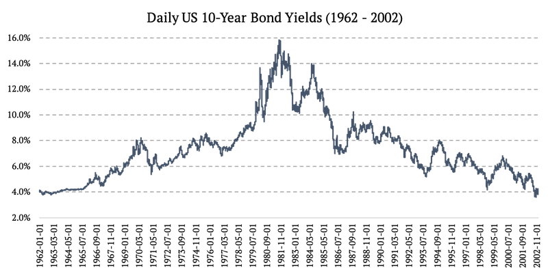
Source: https://fred.stlouisfed.org/series/DGS10
2002 – 2022: IEF ETF (iShares 7-10 Year Treasury Bond ETF)
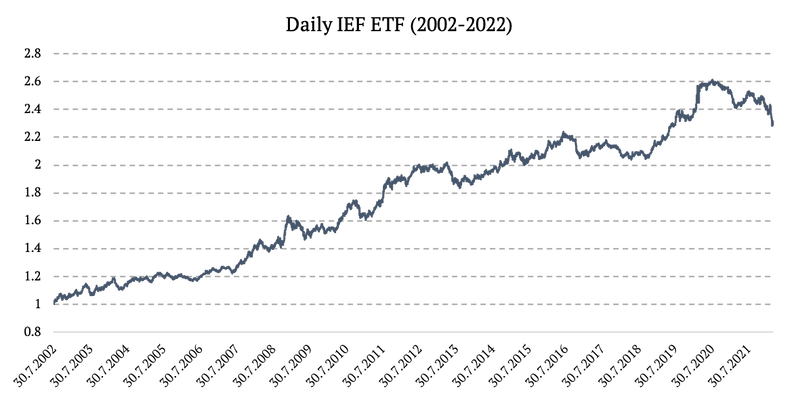
Source: https://finance.yahoo.com/
How to transform Bond Yields into Total Returns
From 1926 to 1962, we worked with monthly yields. First, we needed to transform the bond yields into total returns. Fortunately, once you have a time series of yields, you can quite well approximate also the total return of the respective bond. How? We will show you below. In a simplified way, every single month, a particular bond:
- Earns carry (yield to maturity) fraction equivalent to roughly 1/12 of the YTM
- Is revaluated due to the change in this yield:
- If yields rise, a bond will decline in value by (yield rise)*(duration)
- If yields fall, a bond will increase in value by (yield fall)*(duration)

We already have a time series of bond yields. Now how do we get the time series for duration? Even this, we can approximate. However, first we need to understand and decide whether we want to create a constant duration time series or constant maturity time series.
Constant Duration Bond Series
Constant duration is the easiest case. We simply assume that duration of our bond is constant. For example, we can assume, that the duration of a 10-year US Treasury bond will remain at 8 years.
However, in reality, this often isn’t the case. In reality, if you hold a 10-year US Treasury, and its yield drops significantly, it’s duration will rise. This is caused by the so-called convexity of the bond.
The same applies in reversed direction – if yield on a bond spikes significantly, its duration will drop. Thus, if one wants to maintain “constant duration series” he needs to buy slightly longer or shorter maturities of one particular bond based on how do yields move.
Constant Maturity Bond Series
Constant maturity is the most real case. Most of the ETFs target specific maturity (e.g. 7-10 years), bond futures are also maturity-tied, and many indices and yield data series are also constant maturity time series.
When calculating the total return of the constant maturity bond, we assume the maturity doesn’t change (in our case 10-years for the entire time), however, the duration changes – because yields do change (as described above, due to convexity effect).
Luckily, it’s not that hard to derive duration of a constant maturity bond if we already have a yield data series at hand, which we of course do.
Calculating the Total Return of a Bond
As mentioned above, to calculate the total return for a specific month, firstly, we had to calculate the duration. Fortunately, Excel has an in-build function, MDURATION, which calculates duration from the respective yield and date (we assumed a zero-coupon bond).
Now that we have time series of yields and duration for the bond, let’s calculate the total return for a specific month using the following formula:
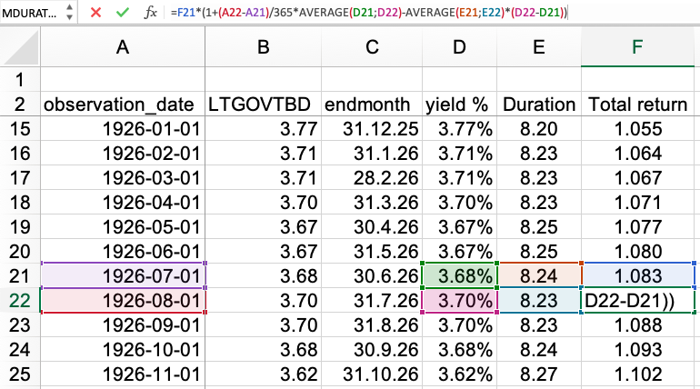
So, the main elements in the formula are: yesterday’s total return (F21), the number of days between the individual months (A22-A21), the average of two consecutive yields (D21;D22), the average of two consecutive values of duration (E21;E22), and the difference between today’s yield and the last yield (D22-D21).
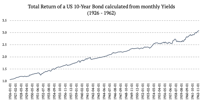
1926 – 1962: Total Return of a US 10-Year Bond calculated from monthly Yields
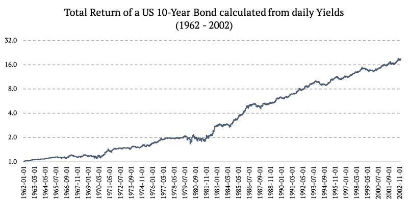
1962 – 2002: Total Return of a US 10-Year Bond calculated from daily Yields (chart below uses log2 y-axis)
Transforming Monthly Data into Daily Data
In the sections above, we created a total return time series for a 10-year US Treasury bond since 1926. However, the part of the data from 1926 until 1962 is at a monthly frequency only. How do we arrive at a daily data then? We have to transform monthly total returns into daily total returns.
As mentioned above, the oldest daily historical data point for US 10-year yields starts in 1962. The older data are monthly only. However, we do have daily data for 3-month T-bills from https://fred.stlouisfed.org/series/DTB3. Let’s now assume T-Bills are highly correlated with Treasuries on an intra-month (daily) timeframe. Or, if we turn it the other way round – can you find anything with daily data from 1954 to 1962 which is more correlated to US Treasuries than US T-bills? Probably not.
Based on this assumption, we are then able to extrapolate the daily volatility from the US 3-month T-bills and apply this volatility intra-month (daily) to our monthly time series of Treasury yields. We call it a “Volatility proxy extrapolation” – and our proxy will be US T-bills.
We divided the monthly 1926-1962 period into two sub-periods: 1926-1954 and 1954-1962. For the first period we applied naïve linear interpolation to arrive at daily data. For the second period we applied our Volatility proxy extrapolation, which we describe below in detail.
Linear interpolation
Unfortunately, there’s no daily proxy for bond volatility before year 1954. Hence, we applied simple linear interpolation on this first sub-period. Every month we calculated the cumulative difference between the two data points to get the daily interest. Then we cumulated the respective interests each day. The main downside is that the resulting equity curve has zero intra-month volatility.
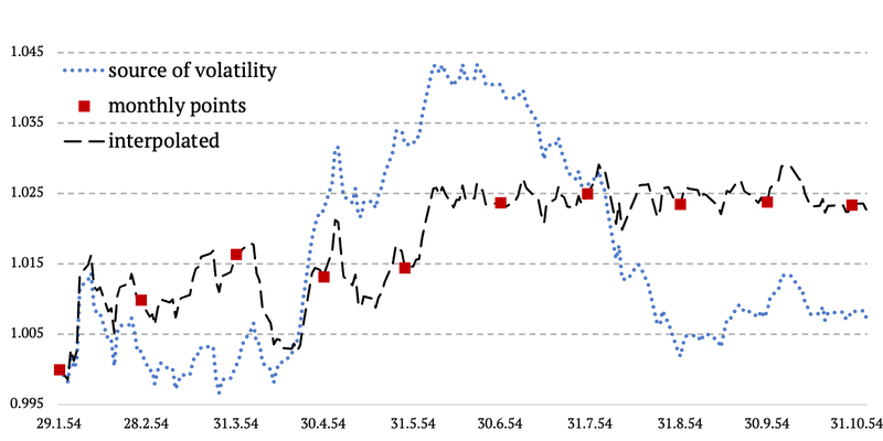
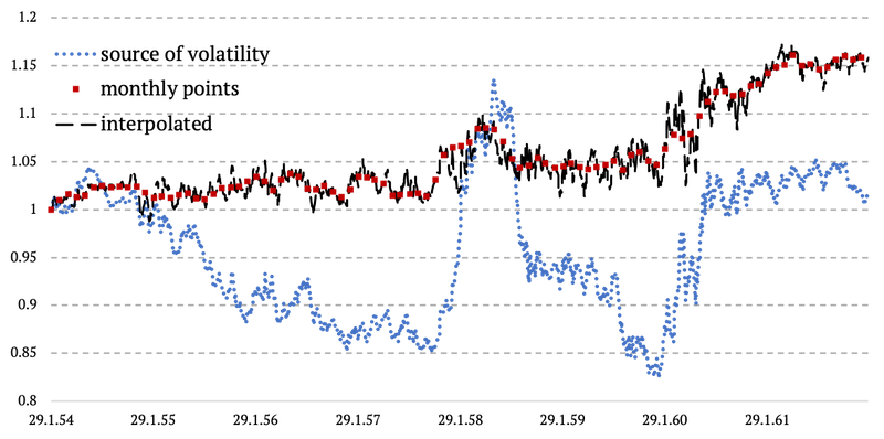
Volatility proxy extrapolation
This time we implemented volatility from an external proxy – US T-bills. Monthly data points of our original data (US 10-year Treasuries, total return) remained untouched. The only thing we changed, is adding and intra-month volatility (daily) with realistic correlation to bond markets (US T-bills).
Each month, we calculated the monthly cumulative difference of the proxy (T-bills) and subtracted it from the monthly cumulative difference of our US 10-year bond and divided it by the number of trading days in the respective month. Thus, getting the daily volatility. The last step was to calculate the cumulative daily return of the US 10-year bond.
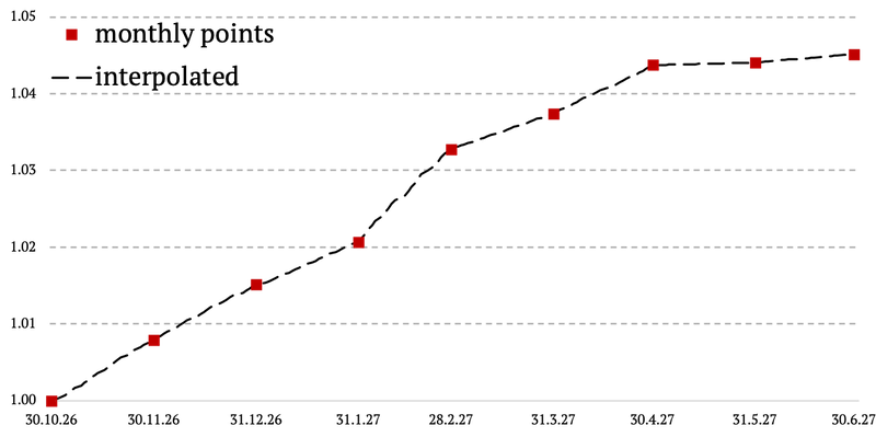
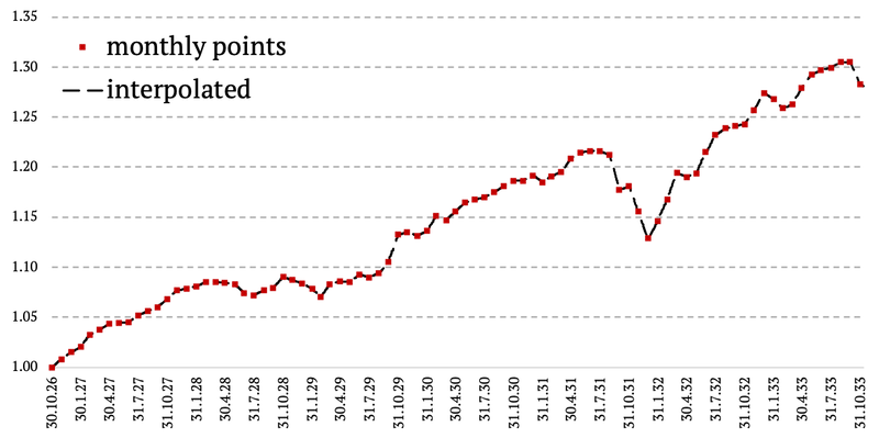
The methodology from above is probably easily understood by a simple chart below. What we basically do in here, is that we copy the daily volatility from the 3-month T-bills and we simply plug it in between two monthly data points of US 10-year Treasuries. And we ensure there are no jumps or gaps in data and everything happens in a linear fashion. See chart below.
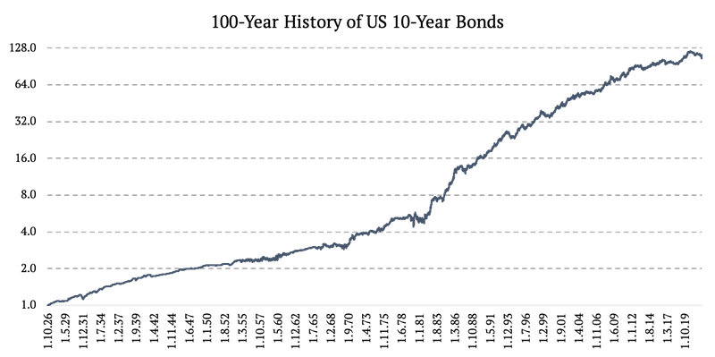
Combining Various Data Sources
Now that we successfully created daily data series from 1926 to 1962 we need to take one last step. That being said, we finally just combined the four periods of different calculations and data sources into one time series:
- 1926 – 1954: Linearly interpolated daily total return,
- 1954 – 1962: Volatility proxy extrapolated daily total return,
- 1962 – 2002: Total return from daily US 10-Year Bond Yields,
- 2002 – 2022: IEF ETF (iShares 7-10 Year Treasury Bond ETF).
The figure below uses log2 y-axis.
Are you looking for more strategies to read about? Sign up for our newsletter or visit our Blog or Screener.
Do you want to learn more about Quantpedia Premium service? Check how Quantpedia works, our mission and Premium pricing offer.
Do you want to learn more about Quantpedia Pro service? Check its description, watch videos, review reporting capabilities and visit our pricing offer.
Do you want algorithmic access to the full Quantpedia database via the API? Subscribe to Quantpedia Pro, ask for an API key, and explore the in/out-of-sample statistics, source academic papers, and code snippets — ideal for quantitative research, systematic trading workflows, and AI model training.
Are you looking for historical data or backtesting platforms? Check our list of Algo Trading Discounts.
Or follow us on:
Facebook Group, Facebook Page, Twitter, Linkedin, Medium or Youtube
Share onLinkedInTwitterFacebookRefer to a friend


