Factor’s Performance During Various Market Cycles
We have already showed How to extend history of any asset, portfolio or strategy to a 100-year long history. We’ve done this by introducing Quantpedia’s Multi-Factor Regression Model, which aims to replicate any portfolio and recreate what its 100-year history would have looked like. The model uses several factors, including Market (U.S. Equities), Bonds, Commodities, Trend factor, etc. In addition to that, we also examined 100 Years of Historical Market Cycles.
Today, we analyze how all the factors we use in our Multi-Factor Regression Model performed during various Market Cycles (in sample), including the Bull/ Bear market, the High/ Low inflation, and the Rising/ Falling interest rates. Further, we also examine the performance of a Balanced Portfolio ETF – AOR, over past 100 years. This is done by creating the Factor AOR, which we constructed using our Multi-Factor Regression Model from AOR ETF. The process of how we reconstructed the 100-year history for AOR ETF is described in detail in our blog.
In addition to a chart comparison of equity curves, we also compare the performance of factor AOR to that of all the factors by means of risk/return tables, i.e. quantitatively. All the tables are sorted based on the Sharpe ratio from the best (at the top) to the worst (at the bottom).
Historical Market Cycles – in sample
We identified eight different combinations of various market cycles related to the state of a) equity markets, b) interest rates, and c) inflation. The detailed methodology on the 100-year history of different market cycles is described in Quantpedia’s primer on market cycles.
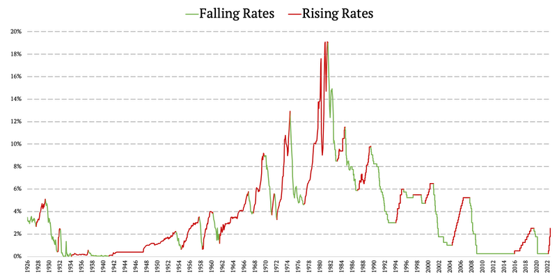
In a nutshell, we firstly isolated various periods of rising and falling equity markets (bull and bear markets). Secondly, we performed the same exercise for interest rates to arrive at periods of rising and falling interest rates. Finally we marked periods of high and low inflation divided by the historical median breakpoint.
Historical market cycles have been identified in sample. This means, we identified these cycles with the benefit of hindsight – already knowing in advance e.g. when exactly a particular bear market started and when the market bottomed to end that bear market. We can then examine performance of any asset over these in-sample market cycles. In our upcoming article, we will identify market cycles also out of sample and compare the results with our in sample analysis.
Factor construction
The full and detailed methodology on how we constructed all of the factors used in today’s article, including their 100-year long daily history, is available in Quantpedia’s factor primer here.
Just briefly, we would like to remind the reader that the factors below are constructed as follows:
- US Equities, US 10y Treasuries, Commodities – as a total return including dividends and coupons (if available)
- US Equity Sectors, World ex US Equities – as an excess return against US Equities
- US BAA Corporates – as an excess return against US 10y Treasuries
- Small-minus-Big, High-minus-Low, Trend – as a standalone long-short strategy


Factors During Bull Markets
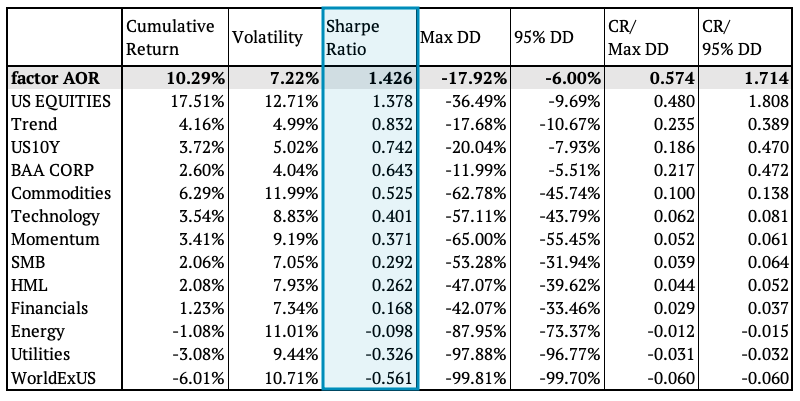
Firstly, we analyze the factors during bull markets. As expected, most of the factors perform well. However, there are a few factors with poor performance during US equity bull markets.

Looking both at the figure above and the table below, the negative performance has been recorded only by World ex-US equities, Utilities and Energy (as a spread against US equities). The worst cumulative return of all factors in bull markets belongs to World ex-US equities spread factor. On the other hand, the reconstructed AOR ETF outperformed all of the model’s factors. A diversification seems to have worked not only theoretically. Additionally, as expected, the U.S. Equities factor performed the best out of all the underlying regression model’s factors.
Factors During Bear Markets
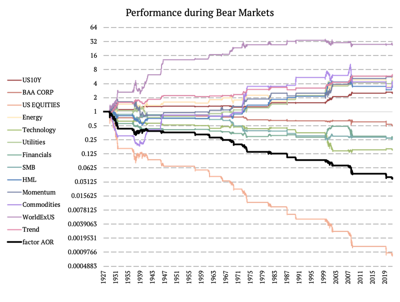
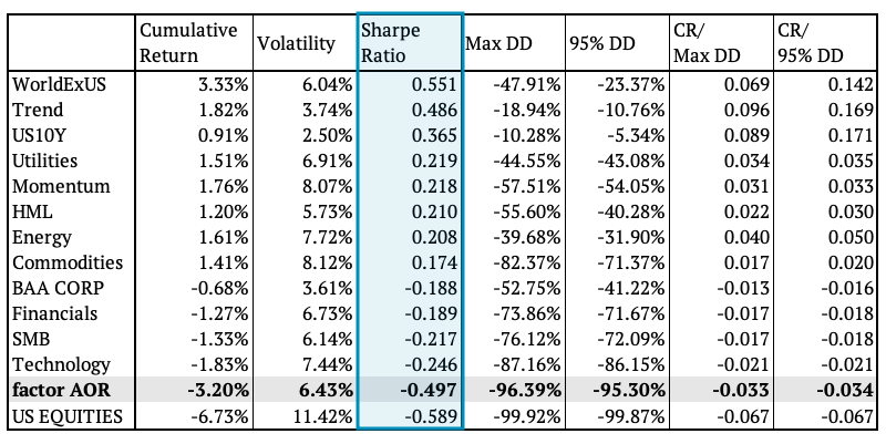
Secondly, we examined how the factors performed during bear markets. We expected opposite results to the bull markets, and the expectation was confirmed in multiple ways. Looking at the Sharpe ratio, the factor AOR ETF performed second to last, as only U.S. equities had worse cumulative return.
The highest Sharpe ratio was surprisingly achieved by World ex-US equities spread factor. It was closely followed by our Multi-Asset Trend-Following strategy (Trend Factor) and by U.S. 10-year bonds (as expected). This is a very interesting result worth a little discussion. If you look at the chart below, you may observe that ex-US equities have actually performed well during US equity bear markets. This outperformance was most pronounced during the 1930s and 1940s. But, even up to this day an excess return of ex-US equities vs. US equities doesn’t perform that bad in recessions! A new defensive asset, maybe?
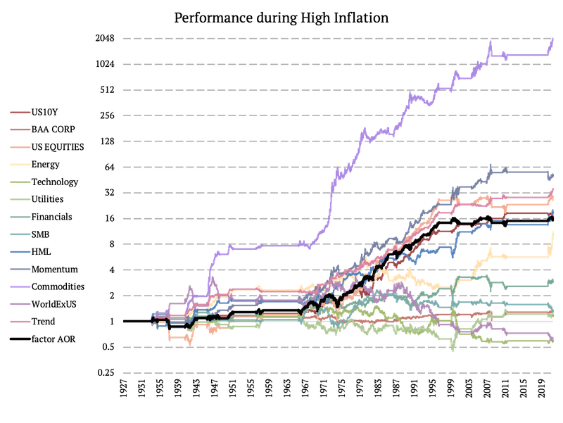
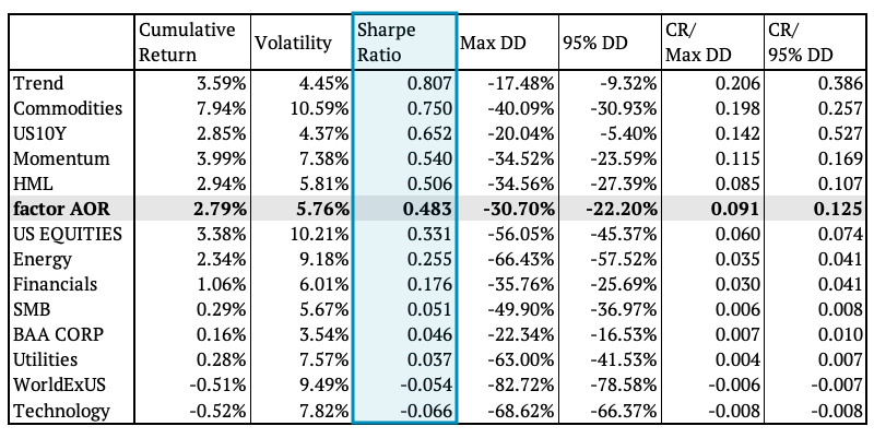
Factors During High Inflation
Next, we examined high vs. low inflation periods. Looking purely at the returns in the figure below, commodities achieved the best result during the high inflation periods. However, they had second to highest volatility resulting in the third best Sharpe ratio. The Trend factor achieved the highest Sharpe ratio. On the other hand, the Technology factor together with the World ex-US equities factor (as a spread against US Equities) recorded the lowest Sharpe ratio and the most significant maximum drawdown.
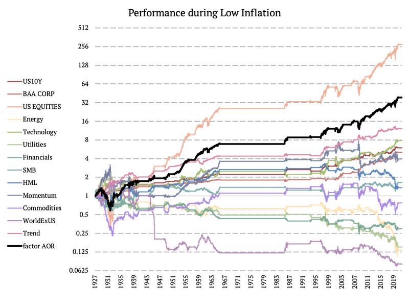
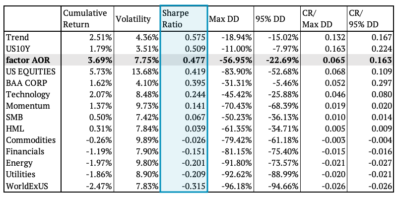
Factors During Low Inflation
On the flip side, U.S. Equities performed the best during low inflation periods. Yet, they had the highest volatility, placing them in the fourth place in our table sorted by Sharpe ratio. The factor AOR is in the third place with the Sharpe ratio of 0.48. The factor with the highest Sharpe ratio is the Trend factor.
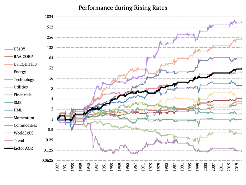
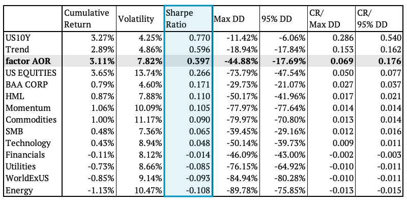
Factors During Rising Rates
Lastly, we compared the performance of our factors during rising and falling interest rates. Again, the Trend factor achieved the highest Sharpe ratio during rising interest rates, even though commodities had the highest cumulative return. The reconstructed AOR ETF ranked fourth according to the Sharpe ratio with the fourth smallest drawdown.

Factors During Falling Rates
Lastly, we examine the factor performance during falling interest rates. U.S. Equities recorded the highest cumulative return and had the fourth highest Sharpe ratio. The factor AOR ETF is placed just above, in the third place. And the U.S. 10-Year bonds sit at the top of the table. On the other hand, Utilities, World ex-US equities and Energy factors (as a spread against US Equities) placed the lowest.

Author:
Daniela Hanicova, Quant Analyst, Quantpedia
Are you looking for more strategies to read about? Sign up for our newsletter or visit our Blog or Screener.
Do you want to learn more about Quantpedia Premium service? Check how Quantpedia works, our mission and Premium pricing offer.
Do you want to learn more about Quantpedia Pro service? Check its description, watch videos, review reporting capabilities and visit our pricing offer.
Do you want algorithmic access to the full Quantpedia database via the API? Subscribe to Quantpedia Pro, ask for an API key, and explore the in/out-of-sample statistics, source academic papers, and code snippets — ideal for quantitative research, systematic trading workflows, and AI model training.
Are you looking for historical data or backtesting platforms? Check our list of Algo Trading Discounts.
Or follow us on:
Facebook Group, Facebook Page, Telegram, Twitter, Linkedin, Medium or Youtube
Share onLinkedInTwitterFacebookRefer to a friend


