Synthetic Lending Rates Predict Subsequent Market Return
It is indisputable that the data are changing financial markets – computing power has increased, allowing to rise the trends of ML/AI and big data (number of possible predictors or granularity) or HFT strategies. Indeed, not all the datasets are worth the time of academics, investors or traders, but we are always keen to analyze the novel and unique datasets. Of course, if we believe that the analysis is worthy of sharing, we are happy to do so. This post offers a shorter version of our newest research about Synthetic lending rates and subsequent market return. We hope that you find it enriching; enjoy the reading!
Introduction
Compared to buying stocks, short-selling them is more complex, and as a result, short-sellers are recognized as sophisticated and informed agents. On the other hand, short selling can be extremely risky since the drawdowns are theoretically unlimited. Moreover, because the agents need to borrow the shares and pay the borrowing fee, it can also be costly. Therefore, one expects that short-sellers are better informed to profit from mispricing. Overall, the literature supports this theorem: Boehmer et al. (2007) show that short interest can be used to predict abnormal returns, where high levels of short interest are negatively correlated with subsequent returns. Gargano (2020) shows that short interest is a bearish indicator, but the author also connects the mispricing signal based on short interest with momentum anomaly and finds that the double sorts are even more profitable than the short interest alone. On the contrary, Hanauer et al. (2020) show that shorting activity is continuously rising and has a weak link to subsequent performance. Therefore, the authors suggest utilizing the change in the short interest or the surprise in short interest defined as the demeaned short interest ratio divided by the standard deviation as a predictor of stock returns.
Even though the research points out that the short-selling might be profitable, there is still one primary concern – shorting constraints. Some stocks might not be available to short at all, and for stocks with high short interest, the shorting costs can be high enough to make the strategy unprofitable. For example, Kim and Lee (2020) show that the performance of long-short strategies significantly drops once we account for the shorting costs.
According to Weitzner (2016), short-selling costs will be higher if negative information is likely to arrive. Moreover, the arbitrageurs do not need to borrow stocks to be able to short them. It is possible to replicate a short position or enter into a “synthetic” short by simultaneously buying a put option and shorting a call option with the same strike price and time to maturity. Based on these synthetic short positions, Weitzner (2016) constructs the term structure of shorting costs using available options and shows how this term structure affects shorting costs and future returns. We partially build on two propositions of the research mentioned above. Firstly, high short-selling costs could point to negative information. In other words, negative sentiment could cause higher shorting costs. However, we are not interested in the cross-section of the returns, but we are interested in whether the aggregate shorting costs for stocks in the market predict the market’s returns. Our research is also based on synthetic short positions (and implied shorting costs), same as in the Weitzner (2016). The synthetic shorting costs data are obtained from Borrow Intensity Indicators by the CBOE.
The borrow intensity equals the risk-free rate minus the lending spread (lending fee) and corresponds to the rebate rate in stock loan transactions. The rebate rate is the rate earned on collateral by borrowers for equity loans. Consequently, the rise (fall) of the borrow intensity corresponds to the decrease (increase) in lending fees or decrease (increase) in shorting costs.
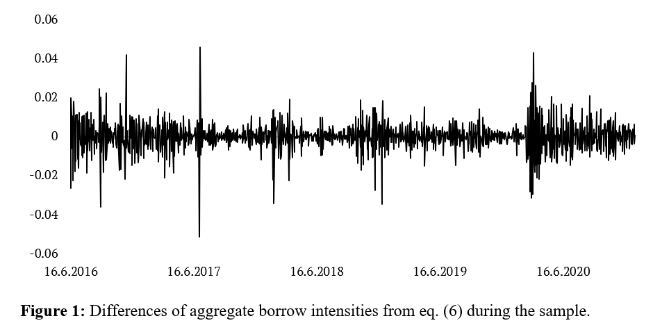
We hypothesize that tight short constraints and higher shorting costs lead to negative sentiment and market returns, and vice versa, lower shorting costs lead to positive sentiment and market returns. In our case, tightening of the shorting costs refers to a situation where the difference of aggregate borrow intensity defined as aggregate borrow intensity at day t minus aggregate borrow intensity at day t-1 is negative. Conversely, the relaxing of shorting costs refers to a situation where the daily difference of aggregate borrow intensity is positive.
So does the theory mentioned above hold in markets? We will find out, but let us talk about borrow intensities, the relationship of intensities and shorting fees, and the overall methodology of the research first.
Data
Synthetic shorting costs data are obtained from Borrow Intensity Indicators by the CBOE. Borrow Intensity Indicators dataset consists of constant maturity synthetic lending rates derived from real-time options analytics based on proprietary analysis of CBOE for 4877 stocks/ETFs. The borrow intensity BI is equal to the risk-free rate minus the lending spread (lending fee, LF) and corresponds to the rebate rate in stock loan transactions:

The rebate rate is the rate earned on collateral by borrowers for equity loans. Consequently, the rise (fall) of the borrow intensity corresponds to the decrease (increase) in lending fees or decrease (increase) in shorting costs. Throughout the paper, we utilize the constant maturities of 45 days. Intraday SPY data are obtained from FirstRate Data and IEF data from Yahoo Finance.
Methodology
First, we clarify why the increase in borrow intensity means that shorting costs have decreased and vice versa. From equation (1), the difference of borrow intensities is equal to:

From day t-1 to day t:

Consequently:

As a result, the rise (fall) of the borrow intensity means that the lending fees decreased (increased).
The aggregate (mean) borrow intensity is calculated as equally weighted borrow intensity of each stock/ETF in the sample at day t:

where BIagg,t is the aggregate borrow intensity, BIi,t is the individual borrow intensity, I is the set of stocks/ETFs for which we have data at time t, and |I| is the cardinality of the set I. The shorting costs data are estimated at a timestamp of 15:57.
Next, we calculate the change in the aggregate intensity at day t:

For robustness, we also estimate the pervasive daily difference in the borrow intensity, which we define as the past 20-days moving average. This rolling moving average of intensity should signal whether the difference is abnormally high compared to the expected value based on current conditions.
The connection between lending rates and market returns
We hypothesize that tighter short constraints (higher shorting costs and demand) lead to negative sentiment and market returns. Conversely, one can also expect that lower shorting costs lead to positive sentiment and market returns. Tightening of the shorting costs refers to a situation where the difference of aggregate borrow intensity is negative (see eq. (4)). On the other hand, the relaxing of shorting costs refers to the positive daily difference of aggregate borrow intensity.
To examine the implications of the rise/fall in intensities/shorting costs, we proxy the market return by the highly liquid SPY ETF. A highly statistically significant positive correlation of 0.137 (t-stats 4.17) between the difference of intensities (and implicitly also lending fees) and subsequent daily return of SPY is found in correlation analysis. On the other hand, SPY’s difference in intensities has only a minor and insignificant correlation with the subsequent SPY return (correlation of 0.023, t-stats -0.49). The finding that equally weighted borrow intensities are correlated with the subsequent return, but the SPY’s intensity is not, confirms that it is better to proxy the aggregate intensity by the equally weighted mean. Value weighted average overweight mega-caps (stock collateral) and should be approximately the same as the borrowing intensity of SPY, which does not seem to have the same predictive power. To summarize, if the borrow intensity decreases (increases), shorting costs increase (decrease). Since the borrow intensity is positively correlated with subsequent market return, we can expect that the return would be negative (positive).
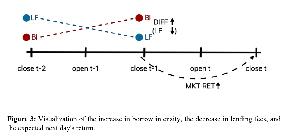
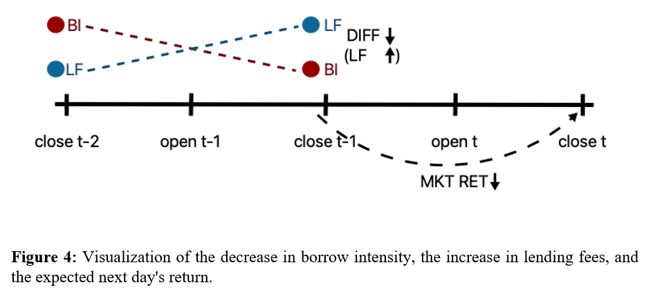
The next question is, does the change in borrow intensities/lending fees economically significantly predict the subsequent market performance? Building on the premise that the short sellers are sophisticated and better-informed investors, the rise (fall) in shorting costs indicating opening (closing) of short positions should relate to lower (higher) next day’s market return.
We empirically examine the relationship between aggregate borrow intensities and subsequent performance by plotting the average market (SPY) returns following -days after the signal (positive or negative change) formation.
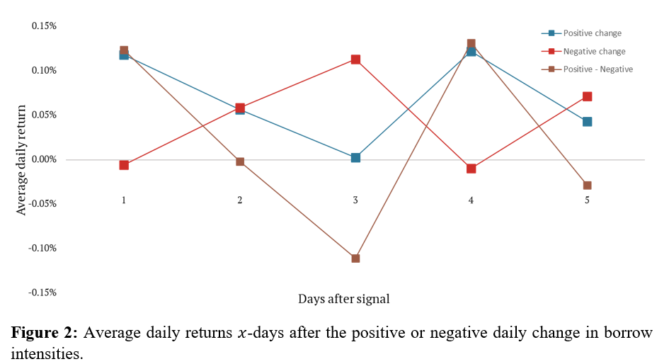
It seems that after a positive change of borrow intensity (decrease of the lending fees), the subsequent daily market return is highly positive, and a negative change of intensity (an increase of the fees) relates to a slightly negative return (see Figures 3 and 4). Nonetheless, the effect reverts over the following days. The performance decreases after the first day for positive change and increases after the initial reaction for negative change. While the average return for a strategy that goes long SPY if the change is positive and shorts SPY if the change is negative is profitable on the first day after signal formation, the next day, the performance is indistinguishable from zero, and it ultimately reverts at the third day. Consequently, the most economically significant effect appears to be the return on the first day after the signal’s formation. The decrease in lending fees predicts a positive return, and the increase in lending fees predicts a negative return. Additionally, based on linear regression with the next day’s SPY return as an independent variable and difference in lending rates as the dependent variable, the relationship seems statistically significant with βBI = 0.22 and t-stats of 4.12.
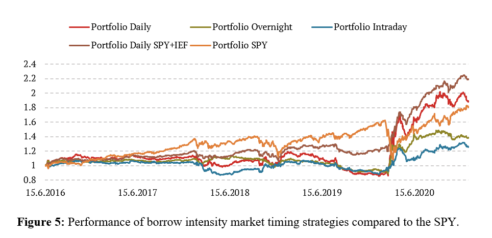
We further verify the economic significance in a simulated trading strategy that buys the SPY at 15:59 if the difference is positive and shorts the SPY if the difference is negative. The positions are held for one day and are closed at 15:58 at next day. The signal is formed at 15:57, and since the latency of CBOE is low, the strategy could have been exploited in practice. In addition, we also examine a long-only strategy that buys the SPY if the difference is positive and buys IEF (Treasury bonds) if the difference is negative.

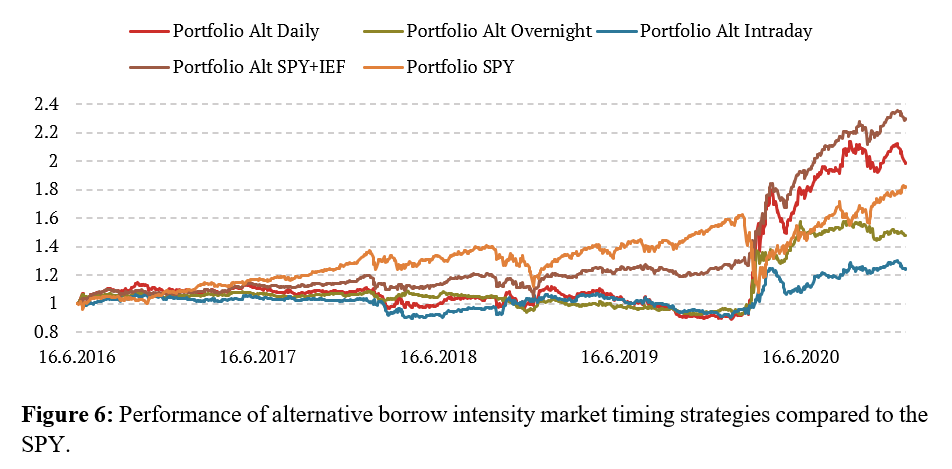
Next, we further examine whether it is better to compare the difference in intensities to the expected value of the intensity. We proxy the expected value by the mean aggregate intensity during the past 20 days (eq. (7)). Comparison of the most recent aggregate and expected borrow intensities should better point to the abnormal increase (decrease) in lending fees than a simple comparison with zero.
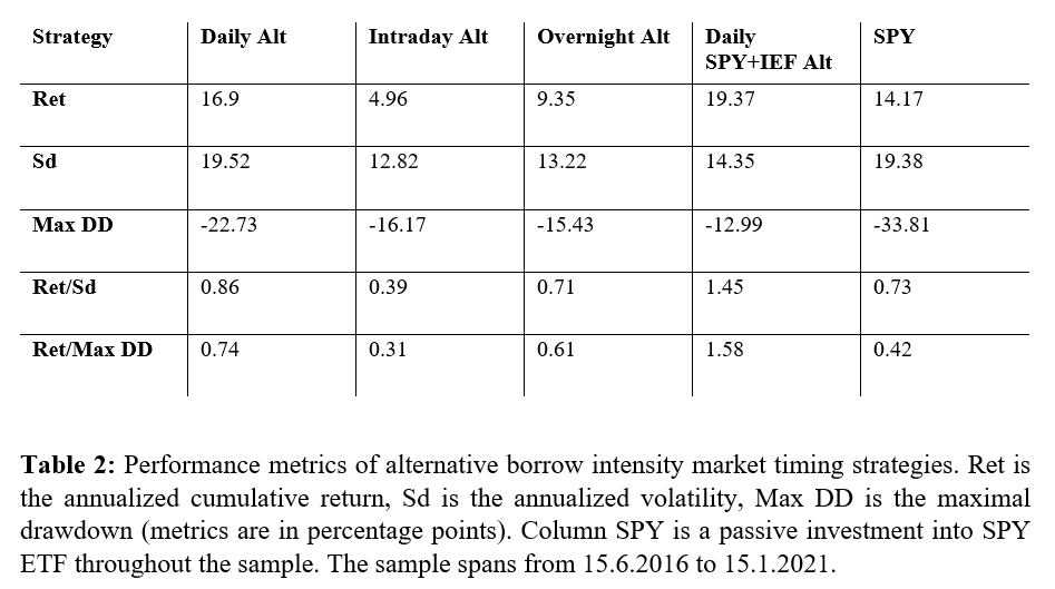
Based on this section, changes in borrow intensities predict the next day’s return – both overnight and intraday components, but the overnight part is more substantial. It seems that the strategies outperform mainly during crises, and there are several periods where the short positions in the market are decreasing the overall performance. The inclusion of IEF instead of shorting seems to alleviate this problem, but still, during calm periods, the strategy can lag the passive SPY investment. However, in the long run, the market timing strategies outperform the passive benchmark. Furthermore, results suggest that it is better to isolate the abnormal change in intensity by comparing the difference in intensities to the prevalent change (or expected change) based on the past one month (approximately 20 trading days).
Robustness
In the previous section, we have found out that the market timing strategies perform better during crises. The sample consists of two well-known market crashes: December 2018 (3.12.2018 till 3.1.2019) and the 2020 Coronavirus Stock Market Crash (19.2.2020 till 3.4.2020). We examine the average daily returns during crises for daily market timing strategy and SPY as a robustness check. The results are summarized in the following table.
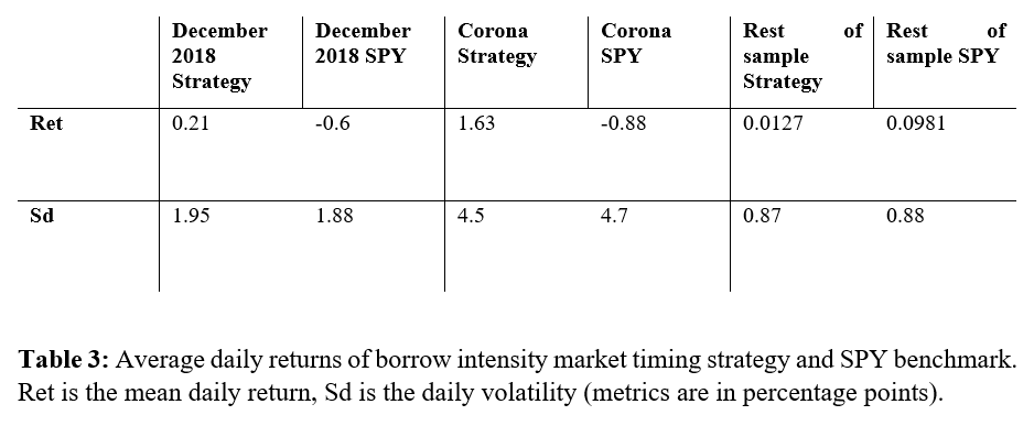
Firstly, the robustness check confirms the evident fact from performance charts, the borrow intensity market timing strategies outperform during crises but lag during “normal” times. Still, the difference during crises is significant enough so that in the long run, the market timing strategy outperforms the passive SPY benchmark. Secondly, these results show that these strategies are potentially good equity market hedges, and perhaps the main benefit of this market timing is during stressful periods.
Conclusion
The difference in synthetic lending rates derived from the options market and provided by the CBOE contains valuable information about the subsequent market’s return. The borrow intensities, closely related to lending fees, predict the following day’s return. If the difference of borrow intensities is positive (negative), it signals a decrease (increase) in lending fees, and the subsequent return tends to be also positive (negative). In line with expectations and previous literature, as the shorting costs rise (fall), negative (positive) sentiment proxied by negative (positive) returns follows. Although the average next day’s average return is highly positive, the effect is short-lived and reversed during the subsequent two days.
A simulated trading strategy that utilizes the intensity-based predictions is economically significant but shines mostly during crises. As a result, the strategy could be a hedge during stressful periods but underperform the passive SPY investment during calm periods. The problem could be partly alleviated by dropping the short leg of the strategy and substituting it with a safe investment to treasury bonds (IEF ETF). Such a strategy seems to compromise exceptional returns during downturns and reasonable returns when SPY is doing well. Still, the performance difference between SPY and market timing strategy during crises is so significant that overall, the market timing strategy fares better.
For additional checks, we show that rather than comparing the difference in lending rates from day to day, it is better to compare it with the expected difference in lending rates proxied by the average difference in lending rates based on the past month. The abnormal difference slightly improves the return and risk profile of the presented strategies.
Empirically the decrease of shorting fees indicates a positive subsequent market return and vice versa. Consequently, the borrow intensity change might be a sentiment indicator. Signaling a positive sentiment after the closing of the short positions (and thus decrease in shorting fees because of the lower demand) or a negative sentiment after the opening of the short positions (and by the increase in short demand, increase in shorting fees). This theory could be supported by the correlation of the difference in borrowing intensities of days t and t-1 and the difference in VIX of days t+1 and t. The difference in borrow intensities is negatively correlated (-0.12, t-stats -4.3) with the VIX (commonly described as the fear index): the increase (decrease) of borrow intensity translates to a decrease (increase) in shorting fees, and as a result, the decrease (increase) in shorting fees signals a subsequent decrease (increase) in the VIX.
Secondly, we have identified that albeit the difference in borrow intensities is positively correlated with the next day’s market return, it is negatively correlated (-0.52 with t-stats -20.898) with the same day’s intraday return. Therefore, the difference in borrow intensities could be related to the short-term reversal, and the exceptional performance after negative returns might be connected with the liquidity provision, which is commonly one of the main explanations of the short-term reversal effect (e.g., Nagel (2011) or Miwa (2018)). We leave this idea for further research.
Author:
Matúš Padyšák, Senior Quant Analyst, Quantpedia.com
Are you looking for more strategies to read about? Sign up for our newsletter or visit our Blog or Screener.
Do you want to learn more about Quantpedia Premium service? Check how Quantpedia works, our mission and Premium pricing offer.
Do you want to learn more about Quantpedia Pro service? Check its description, watch videos, review reporting capabilities and visit our pricing offer.
Do you want algorithmic access to the full Quantpedia database via the API? Subscribe to Quantpedia Pro, ask for an API key, and explore the in/out-of-sample statistics, source academic papers, and code snippets — ideal for quantitative research, systematic trading workflows, and AI model training.
Are you looking for historical data or backtesting platforms? Check our list of Algo Trading Discounts.
Or follow us on:
Facebook Group, Facebook Page, Telegram, Twitter, Linkedin, Medium or Youtube
Share onLinkedInTwitterFacebookRefer to a friend


