Trading the Spread: Bitcoin ETFs vs. Cryptocurrencies Infrastructure ETFs
In this study, we explore the application of simple spread trading strategies using Bitcoin ETFs and cryptocurrency infrastructure ETFs—two highly correlated asset classes due to the broader influence of cryptocurrency market movements. Given their strong relationship, this setup provides a compelling case for implementing pair trading strategies based on mean reversion principles. Building on our previous work, How to Build Mean Reversion Strategies in Currencies, we adapt and extend these models to the cryptocurrency ETF space, demonstrating their broader applicability beyond traditional currency markets. Specifically, we test two sub-methods of mean reversion: linear and exponential. Our goal is to offer a practical example of how traders can leverage these techniques across different asset classes.
Introduction
Pair & Spread Trading
Pair trading is a market-neutral trading strategy that involves taking opposing positions in two correlated assets. The goal is to profit from the relative movement between the two assets, rather than from the direction of the market as a whole. First, we need to identify two assets that have a strong historical correlation (or at least there is expected correlation because of causality). This could be stocks, ETFs, commodities, or other financial instruments. In our article, we choose a Bitcoin ETF and a crypto infrastructure ETF, as revenue of crypto infrastructure is directly related to the underlying cryptocurrency they operate with (for example revenue of Bitcoin miners is tied to the price of Bitcoin itself).
When we choose our correlated assets, we need to construct a spread. That means that we take a long position in one of them and hedge it with a short position in the other. To make a profit, the long position is taken on higher beta asset (in our case Bitcoin ETF) and short position is taken on the other asset (crypto infrastructure ETF).
Mean reversion
To make pair and spread trading work, we need to have mean reverting assets. By that we mean assets that after diverting from their average or historical means over time return to those expected values. For example, if the price of a stock falls far beyond its historical average, it might be considered oversold. Mean reversion theory suggests that after such a deviation, the price will tend to correct itself, moving back toward its average level.
BLOK & BITO
For this pair trading (mean reversion) strategy, we are going to use BITO and BLOK ETF. BITO ETF (ProShares Bitcoin ETF) is a fund designed to replicate Bitcoin’s behavior through trading Bitcoin futures. The fund maintains these futures independently of futures price fluctuations. Why did we pick BITO ETF and not spot Bitcoin ETFs? The main reason is data availability, as BITO had an inception date in 2021, while spot Bitcoin ETFs started in 2024. This gives us a longer backtest period over which we can analyze data. BLOK ETF (Amplify Transformational Data Sharing ETF) is a growth-oriented fund with a focus on transformative data-sharing technologies, i.e. cryptocurrency infrastructure. Seventy percent of the fund is allocated directly to infrastructure, while thirty percent is invested in companies that have partnered with or invested in such firms. Once again, we picked the BLOK ETF and not alternatives, as this is the ETF with the longest data history.
Recently, Yahoo Finance discontinued free end-of-day data downloads. As a result, we recommend sourcing data from our preferred provider, EODHD.com – the sponsor of our blog. EODHD offers seamless access to +30 years of historical prices and fundamental data for stocks, ETFs, forex, and cryptocurrencies across 60+ exchanges, available via API or no-code add-ons for Excel and Google Sheets. As a special offer, our blog readers can enjoy an exclusive 30% discount on premium EODHD plans.
Constructing spread
To establish a spread, it is usually better to select an asset with higher returns for the long position and hedge it with a lower-yielding asset by creating a short position. Usually, when 2 assets are available, the higher beta asset is the more profitable, while the lower beta asset (less volatile) is the one that’s suited for the short leg of the spread. In our case, we utilize the BITO ETF for long positions and the BLOK ETF for short positions. The rationale behind this setup is that the price of companies providing infrastructure related to Bitcoin is correlated with the price of Bitcoin, although not exclusively driven by it, therefore with a lower beta.
There are various methods to construct a spread. One possibility is to create a beta-neutral spread when the portfolio weight between the long and short legs is different (for example, 50% long vs. -100% short if the long leg has a significantly higher beta than the short leg). In this article, we opt for a simple dollar-neutral spread – a 100% long position combined with a 100% short position, as the beta of both ETFs is close to 1.0 (BLOK ETF has a beta of 0.93 against BITO ETF). When beta sufficiently deviates from 1, it is better to pursue alternative strategies (not dollar-neutral strategies).
A quick word about total portfolio leverage: Our maximal position in the spread will be 100% long BITO and 100% short BLOK, which means that our total portfolio leverage doesn’t exceed 200% of the portfolio. This allows us to easily hold overnight positions in the spread in most of the margin accounts offered by regulated brokers.
The final consideration when trading short positions on ETFs is the associated costs, which can become substantial with frequent trading and extended holding periods. These costs will be factored into our models and will be represented by AMERIBOR rates during the trading period.
Linear and Exponential strategies
After constructing a spread, it is essential to establish the trading rules of the strategy we will be employing.
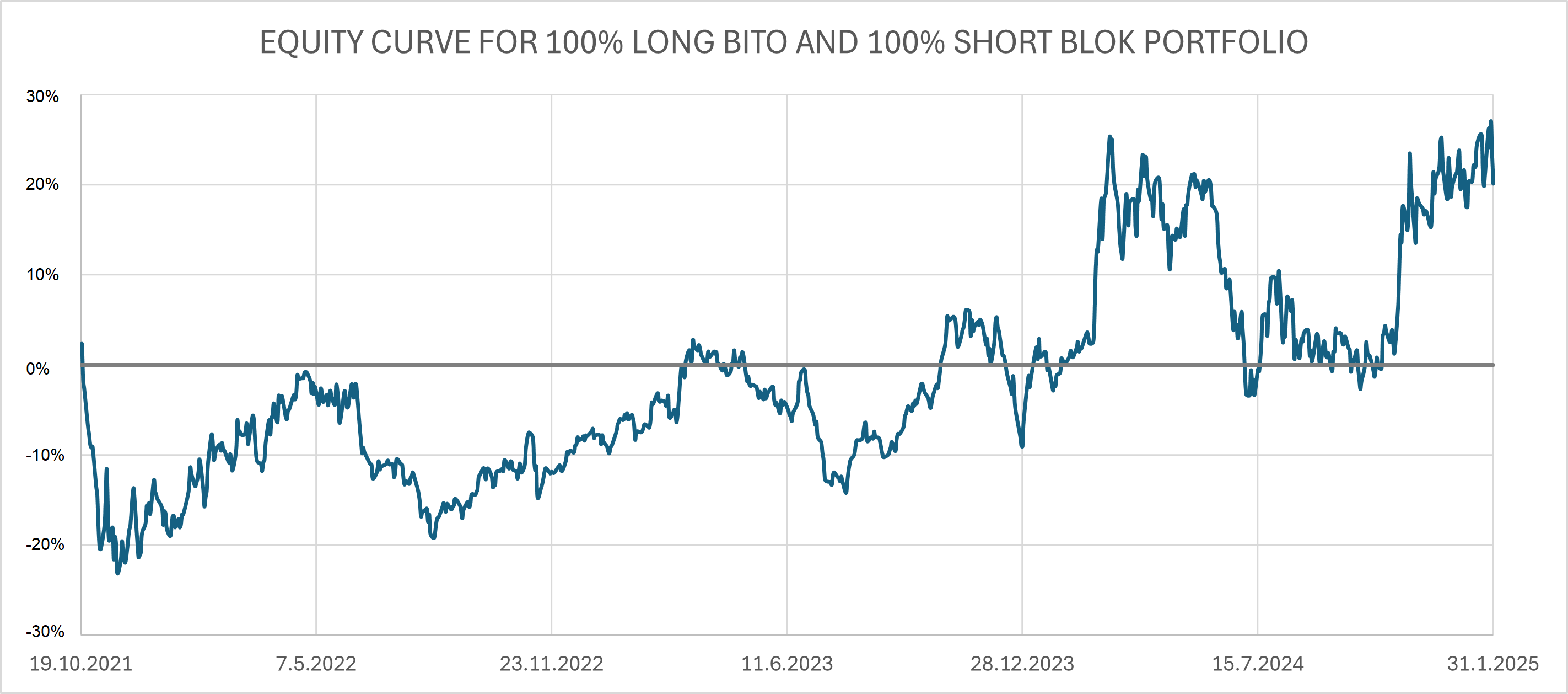
Upon examining the equity curve of this spread, we can infer that it oscillates approximately around zero, albeit with a small upward trend. The small upward trend visible in the data is however highly sensitive to the start and end of the data set (if we remove last 3 months of the data, the upward trend in data disappears). Our simplified working hypothesis for this article is that the spread remains to mean revert towards 0, but there are a lot of methods how to deal with a trending spread (the easiest one is not to use a neutral spread, but a beta neutral spread).
As the spread obviously reverts to the mean, it enables us to implement a set of straightforward strategies based on the distance of the equity curve from the value of 0%.
Two strategies we are going to discuss today are linear and exponential (we discussed both variations in our previous blog How to Build Mean Reversion Strategies in Currencies). What does this mean in terms of trading spread? These strategies involve assessing the deviation of the equity curve from 0% to establish the optimal position in the spread. In linear strategy, for instance, if the equity curve is 20% below 0%, we establish a 20% long position in the spread for a day or month. Conversely, if the equity curve is 20% above 0%, we establish a 20% short position in the spread, and so on. The exponential strategy follows a similar principle but with a greater degree of leverage introduced by greater deviations. If the equity curve is 20% below (above) 0%, we open a 40% long (short) position. Similarly, if the equity curve is 30% above (below) one, we open a 90% short (long) position. However, it is important to note that the exponential strategy entails higher risk compared to the linear strategy.
Daily rebalancing
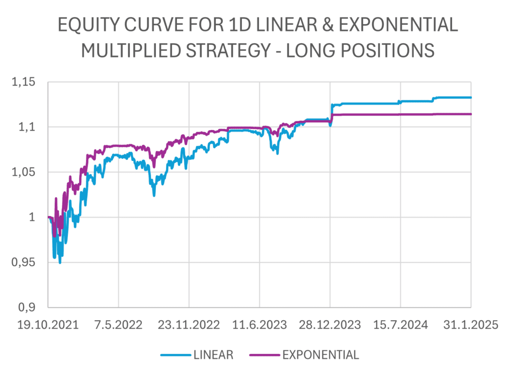
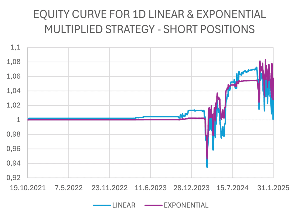
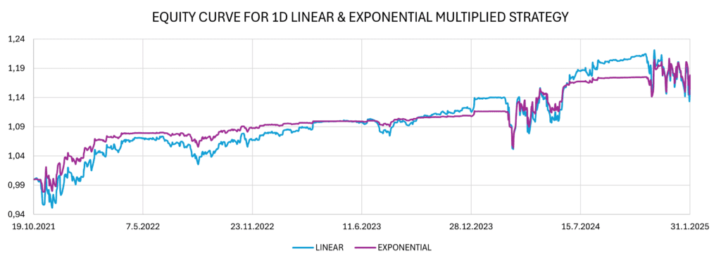
The figures below show the implementation of linear and exponential strategies with daily rebalancing. The strategies consist of a combination of long trades and short trades, which can be seen listed separately.
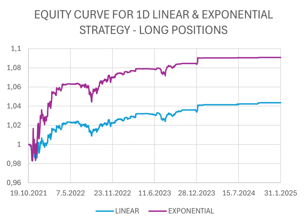
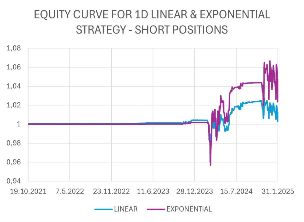
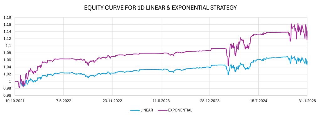
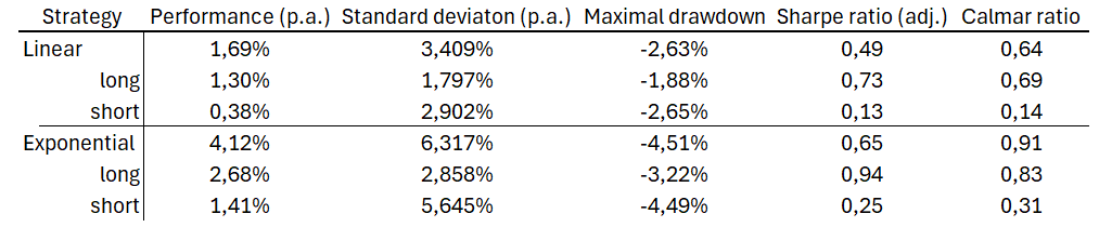
We observe that while exponential strategies yield higher returns, they are also associated with increased risk, as indicated by standard deviation and maximum drawdown. However, when we adjust returns for risk using the adjusted Sharpe ratio and Calmar ratio, we find that the in overall, the exponential strategies, along with its long and short components, yields better results.
These strategies present a minor issue regarding the percentage of the portfolio allocated. Most of the time, they are under-invested. In this case, we have not allocated more than 30% of the capital in linear strategy (as spread rarely goes over 30% or under -30%), and we can address this by multiplying the weights by a factor of 3, allowing room for higher portfolio allocations. In the future, when the difference between the equity curve and the 0% line exceeds 33.3%, we can cap allocations at 100%. A similar situation occurs in exponential strategies (where we are too under-invested, albeit not to such a degree), where we can use a factor of 1.25.
In these instances, we observe that although the yield is higher, risk-adjusted ratios indicate that the trade-off between the increased return and the consequent rise in risk may not be justified.
Monthly rebalancing
Another approach to build a basic mean reverting spread/pair trading strategy is by focusing on the rebalancing period. Previously, we presented results for 1-day trades. However, trading assets daily can introduce numerous undesirable issues. The primary concern is the cost (slippage + transaction fees) associated with buying and selling. This becomes problematic when the trading volume is very low, potentially causing us to lose most, if not all, of the profit generated by our strategy, even after accounting for one of the most significant costs – short expenses.
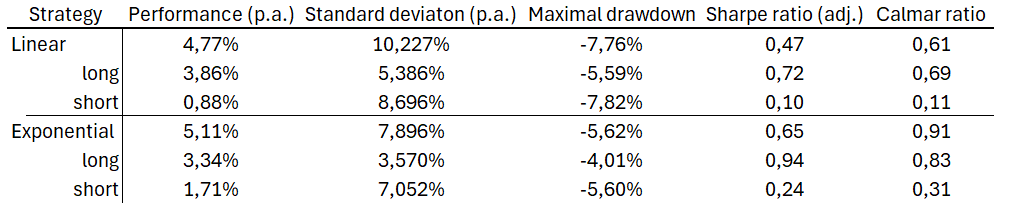
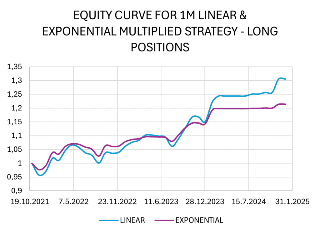
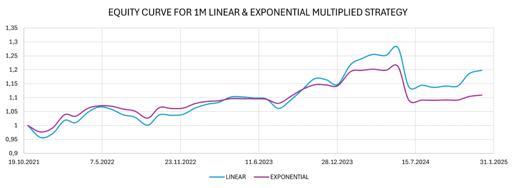
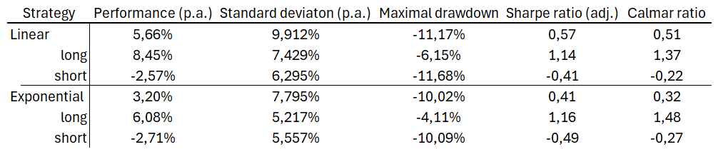
Consequently, we applied the same approach as in 1-day trades and generalized the results for a 1-month rebalancing period. We developed linear and exponential strategies without multiplying the calculated weights, and the results are presented in the figure and table below.
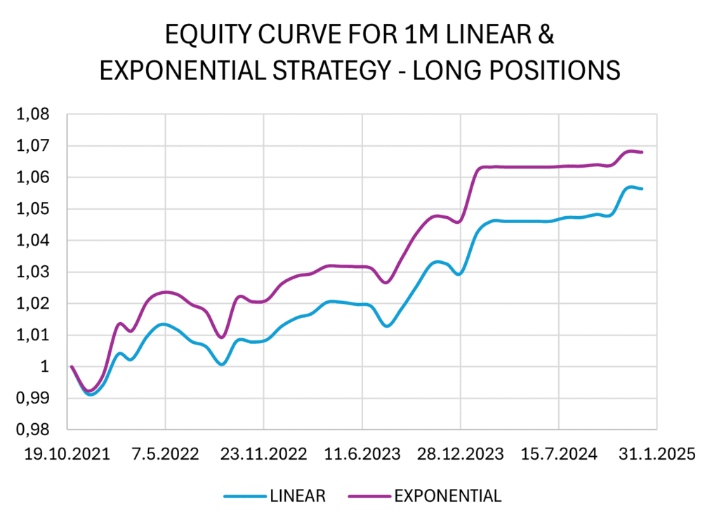
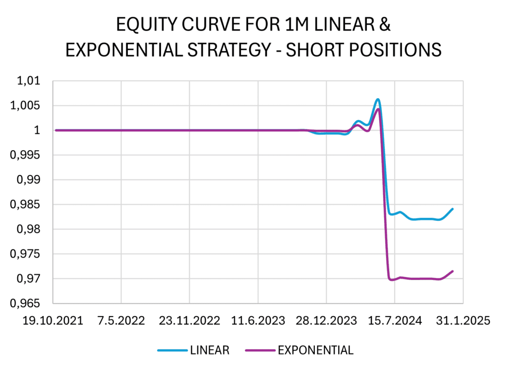
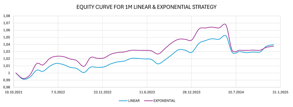
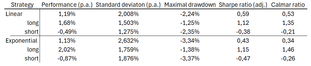
We observe that the yield of both strategies is very similar, but all indicators suggest that the linear strategy is more successful in this case. Additionally, it is important to note that the short positions in both strategies generated losses. The spread between BITO and BLOK ETFs gradually increased in the sample period, as the BITO ETF had a higher beta than BLOK ETF and captured more from the upside movements in cryptocurrencies. One possibility for the improvement of the performance for the short positions is not to use a normalized dollar-neutral spread (100% long ETF vs. 100% short ETF) but rather a beta-neutral spread (as we have already mentioned in the “Constructing spread” section).
In both strategy variants (linear and exponential), we encounter the same issue as before: we do not use higher percentages of allocations, which results in small total performance. We deduced that multiplying the allocation weights by a factor of 5 for the linear strategy and by a factor of 3 for the exponential strategy allows for sufficient space to avoid full allocation towards our spread and increase the total returns.
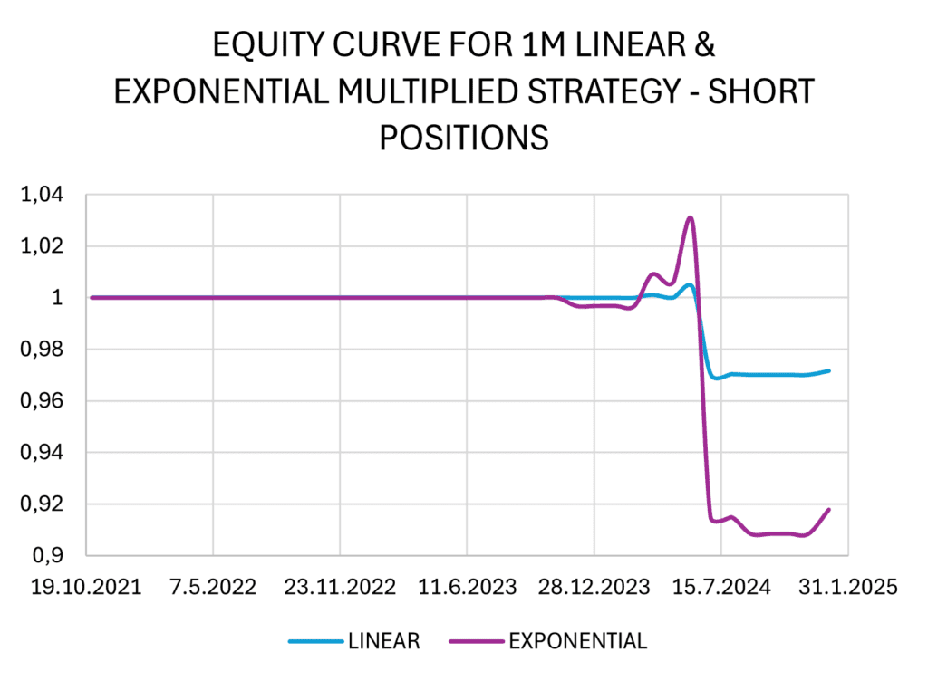
As anticipated, the loss generated by short positions persists, as the weights are merely multiples of those in the original model. However, the losses in the short positions can be a consequence of an ongoing cycle, which has not yet been concluded. Cryptocurrency prices may have temporarily overshot their expected internal values, and simultaneously, many crypto-related corporations can struggle to maintain their financial health.
Conclusion
In this article, we employed one of the fundamental principles of technical investing – mean reversion. Our focus was on its application in spread trading on cryptocurrency-related ETFs. The dollar-neutral spread we constructed long positions on the BITO ETF (Bitcoin futures) and short positions on the BLOK ETF (cryptocurrency-related infrastructure).
After constructing the spread, we focused on the most basic trading strategies – opening long positions when the spread indicated the undervaluation of Bitcoin in contrast with related crypto-infrastructure companies and opening short positions when we observed perceived overvaluation of Bitcoin. Subsequently, we presented linear and exponential strategies based on daily and monthly rebalancing and introduced strategies that involved multiplying the calculated allocation weights to increase yield without significantly increasing risk.
We discovered that in daily rebalancing, the exponential strategy provided better risk-adjusted returns, with the best results achieved using the exponential 1.25-times weights strategy, yielding an annualized return of 5.11%. For monthly rebalancing, the best-performing strategy focused on opening long-only spread positions with a 5-times weights linear strategy, resulting in a yearly yield of 8.45%.
In summary, trading spreads on cryptocurrency-related ETFs could provide an opportunity to diversify a portfolio containing other assets that are not extensively correlated with the given spread. This article presented methods that were not the most sophisticated, nor were the strategies optimized for risk-adjusted returns. These criteria could be added and explored later, but for now, we aimed to focus on simplicity and introduce a set of essential algorithms for mean reversion strategy in cryptocurrencies and related industries that can be improved later on.
Author: David Belobrad, Quant Analyst, Quantpedia
Are you looking for more strategies to read about? Sign up for our newsletter or visit our Blog or Screener.
Do you want to learn more about Quantpedia Premium service? Check how Quantpedia works, our mission and Premium pricing offer.
Do you want to learn more about Quantpedia Pro service? Check its description, watch videos, review reporting capabilities and visit our pricing offer.
Are you looking for historical data or backtesting platforms? Check our list of Algo Trading Discounts.
Would you like free access to our services? Then, open an account with Lightspeed and enjoy one year of Quantpedia Premium at no cost.
Or follow us on:
Facebook Group, Facebook Page, Twitter, Linkedin, Medium or Youtube
Share onLinkedInTwitterFacebookRefer to a friend