
Front-Running Seasonality in US Stock Sectors
Seasonality plays a significant role in financial markets and has become an essential concept for both practitioners and researchers. This phenomenon is particularly prominent in commodities, where natural cycles like weather or harvest periods directly affect supply and demand, leading to predictable price movements. However, seasonality also plays a role in equity markets, influencing stock prices based on recurring calendar patterns, such as month-end effects or holiday periods. Recognizing these patterns can provide investors with an edge by identifying windows of opportunity or risk in their investment strategies.
In this study, we combine our knowledge obtained from articles such as Trader’s Guide to Front-Running Commodity Seasonality (how front-running affects commodity seasonality patterns), Market Seasonality Effect in World Equity Indexes (calendar-based anomalies across global equity markets), January Effect Filter and Mean Reversion in Stocks (well-known phenomenon where small-cap stocks often outperform in January) or 12-Month Cycle in Cross-Section of Stock Returns (the cyclical nature of returns across stocks over a yearly horizon). These insights underline the importance of understanding seasonality in both commodities and equities, offering investors the tools to refine their strategies and capitalize on predictable market behaviors.
Methodology
In this study, we utilized the daily adjusted closing prices of the 9 sectors of the S&P 500 index (ETFs) for all analyses. These sectors include XLB (materials), XLE (energy), XLF (financials), XLI (industrials), XLK (technology), XLP (consumer staples), XLU (utilities), XLV (health care), XLY (consumer discretionary). However, the analysis was conducted using only the final value of each month.
The ETFs are adjusted for dividends and splits, ensuring that historical prices have been modified to reflect dividend payouts and stock splits. This adjustment provides a more accurate representation of the ETF’s performance over time by accounting for total returns, including reinvested dividends, and by correcting for price changes due to splits. Using these adjusted prices is crucial for precise historical performance analysis and strategy comparison. The data were sourced from Yahoo Finance and span the period from December 22, 1998, to September 5, 2024.
However, recently, Yahoo Finance discontinued free end-of-day data downloads. As a result, we recommend sourcing data from our preferred provider, EODHD.com – the sponsor of our blog. EODHD offers seamless access to +30 years of historical prices and fundamental data for stocks, ETFs, forex, and cryptocurrencies across 60+ exchanges, available via API or no-code add-ons for Excel and Google Sheets. As a special offer, our blog readers can enjoy an exclusive 30% discount on premium EODHD plans.
True seasonality
Firstly, we constructed a strategy based on a true seasonality. In this method, ETFs are selected for purchase in the following month based on their previous performance during that specific month. For example, at the end of December, an investor selects ETFs for January by evaluating their performance in the previous January and choosing the most effective ones for the long side (alternatively, the least effective for the short side).
Based on these rankings, we selected the best-performing ETFs from the same month of the previous year, corresponding to the upcoming month. This process was repeated monthly. For comparison, we also constructed a benchmark comprising the average performance of all ETFs for each month.
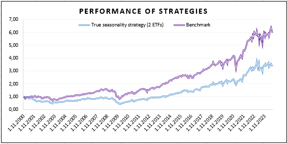
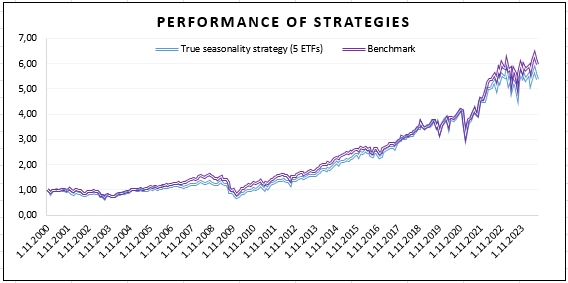
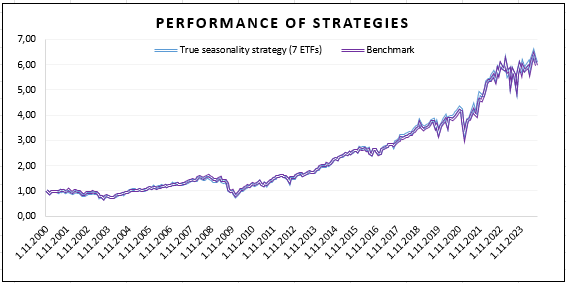

According to Table 1, the results achieved by the true seasonality strategy are, at best, comparable to those of the benchmark, as is evident from the graphs in Figure 1. Regardless of the number of ETFs selected for a long position, the strategy remains inefficient (on the performance and also on the return/risk basis).
Additionally, we calculated also the long-short versions of this strategy to determine whether a short or long position would be more appropriate for each ETF. However, it appears that short positions are ineffective in this strategy, and only long positions are reasonable.
Front-running strategy
Due to favorable results achieved by the front-running strategy based on commodity sectors presented in the article Trader’s Guide to Front-Running Commodity Seasonality, we decided to apply a similar front-running approach to US stock sectors. For example, at the end of December, an investor selects ETFs for January by assessing their performance from the previous February and choosing the top-performing ones. However, unlike the original approach, which selects ETFs for long/short positions based on the comparison of the performance in month t-11 to the performance over the last 12 month period (time-series approach to the seasonality), our approach for equity sectors uses the cross-sectional approach to seasonality – in the examined month, we compare the performance of sector ETFs to each other.
The front-running approach to ETF sector seasonality capitalizes on the behavior of investors who follow established seasonality patterns. Knowing that certain investments perform well in a specific month, it can be more profitable to buy these assets one month earlier, before the majority of investors act. This early positioning anticipates the pressure from increased demand, which is likely to drive asset prices higher, potentially leading to greater returns.
Therefore, as with the true seasonality approach, we rank the ETFs using the same pattern, maintain long positions in the top-ranked ETFs, and rebalance monthly. The only modification is that the month used for ETF selection is shifted forward by one month. By using this approach, the strategy achieved the best results by holding two ETFs in long positions. As before, we compare the strategy’s performance against a benchmark.
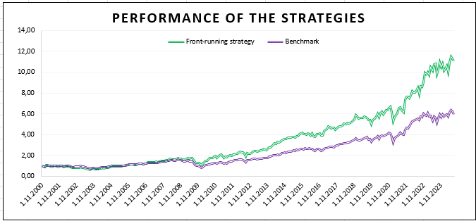
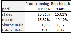
At first glance, it is evident from the graph in Figure 2 that the Front-running strategy using 2 ETFs for long positions outperforms the benchmark, particularly since 2009. This conclusion is also supported by the data in Table 2. Although the Front-running strategy exhibits a higher standard deviation compared to benchmark, its superior returns result in a more favorable Sharpe Ratio. Additionally, the higher Calmar Ratio highlights the efficiency of this strategy. All of the other variants, be it 1, 3, 4, 5, 6, or 7 ETFs in long leg beat the benchmark with a wide margin, too.
Additionaly, we calculated the Alpha of the Front-running strategy relative to the benchmark, which is the same as in previous analyses (equally weighted universe of sector ETFs).
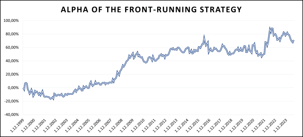
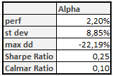
The performance of the Alpha of the Front-running strategy relative to the benchmark, illustrated in the graph in Figure 3, shows a tendency to grow with no significant drawdowns. This reflects the efficiency and outperformance of the strategy compared to the benchmark.
Seasonality sensitivity
In the final part of this study, we investigated whether there is any seasonality sensitivity in US stock sectors, in other words, whether specific months months exhibit a stronger seasonality effect than usual. This analysis was inspired by the Seasonality Analysis by Quantpedia, which can also be applied to daily data.
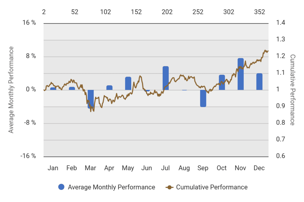
Since this research is based on monthly data, the calculations must be performed manually. How it worked? We took the monthly performance of the front-running seasonal strategy from the previous chapter (Figure 2) and analyzed what’s the performance contribution of the each month into the performance. The resultant sensitivity chart looks like this:
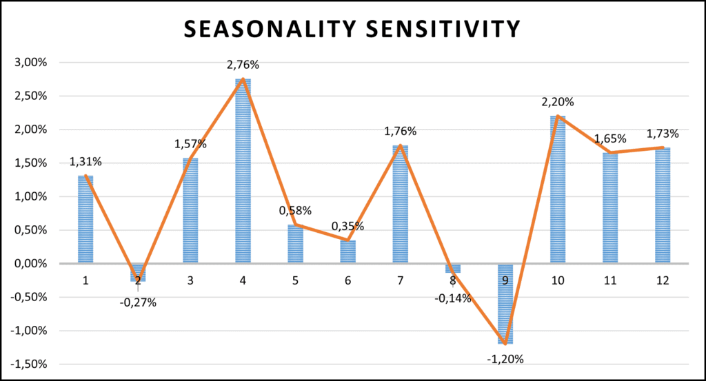
From the graph in Figure 5, we can hint at two well-known effects and trends. The higher performance in the period between October and April may be attributed to the market seasonality effect, which is detailed in the Market Seasonality Effect in World Equity Indexes. Another possible pattern is quarterly seasonality, as described in Momentum Seasonality and Investor Preferences, which can be seen as the higher performance at the beginning of each new quarter, specifically in January, April, July, and October. However, we want to avoid drawing strong conclusions from this analysis as the resultant sensitivity chart could still be a coincidence.
Conclusion
The behavior of investors focusing on seasonal patterns truly impacts the market in the month preceding the expected seasonality. By considering this phenomenom and incorporating it into our strategy, we can create an effective approach that outperforms not only the true seasonality strategy, but also the benchmark. The alpha of the front-running strategy is also positive, reflecting its ability to beat the benchmark. The seasonal sensitivity analysis hints two more patterns, however, we want to avoid drawing strong conclusions at this moment and may revisit this topic in the future.
Author: Sona Beluska, Junior Quant Analyst, Quantpedia
Are you looking for more strategies to read about? Sign up for our newsletter or visit our Blog or Screener.
Do you want to learn more about Quantpedia Premium service? Check how Quantpedia works, our mission and Premium pricing offer.
Do you want to learn more about Quantpedia Pro service? Check its description, watch videos, review reporting capabilities and visit our pricing offer.
Are you looking for historical data or backtesting platforms? Check our list of Algo Trading Discounts.
Would you like free access to our services? Then, open an account with Lightspeed and enjoy one year of Quantpedia Premium at no cost.
Or follow us on:
Facebook Group, Facebook Page, Twitter, Linkedin, Medium or Youtube
Share onLinkedInTwitterFacebookRefer to a friend


