A Balanced Portfolio and Trend-Following During Different Market States
What’s the performance of a balanced portfolio during rising rates? How does it behave when inflation is high? What about a combination of these market states? And how do trend-following strategies fare in such an environment? These and even more questions we will attempt to resolve in our today’s article. We will be looking at different market cycles and how a balanced portfolio and a typical trend-following strategy perform over these different market states.
In our recent article, we identified periods of bear vs. bull market, high vs. low inflation, and falling vs. rising interest rates over the past 100 years. In addition, we also examined the performance of bonds, stocks, and commodities during each of these periods and their combinations. The aforementioned market states were identified with the benefit of hindsight, which is very useful for everyone who has a specific view on the current market cycle. They can then easily examine which assets perform best and worst during a specific market state.
This article builds on top of the foundation set by our previous article. We examine the performance of a Balanced Portfolio during various stock market, inflation, and interest rate phases. A balanced portfolio will be represented by a well-known ETF with abbreviation AOR US – a benchmark for balanced funds. However, the AOR ETF history stretches back only to 2008. We will first have to extend the history of AOR to 100 years into the past. Luckily, we’ve already done this exercise recently and we created a 100-year long history of daily data for AOR US – balanced ETF – using Quantpedia’s proprietary multi-factor regression model.
A Balanced Portfolio over 100 Years of different Market Cycles
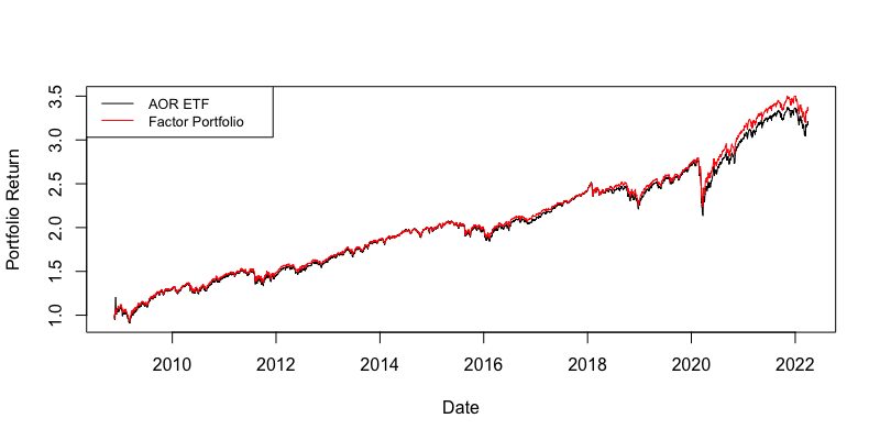
As we’ve already mentioned in our flagship portfolio replication article, the first step of our analysis is to replicate the AOR ETF with factors and extend its history to 100 years of daily data. The following figures show firstly the identified factors which replicate AOR well and, secondly, the performance of the original AOR ETF and the new portfolio, which replicates the AOR ETF using four factors.
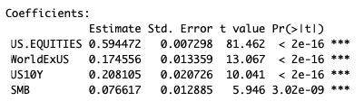
We have replicated AOR US with 4 factors as stated above and this is how the resulting replication looks:
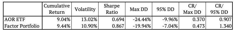
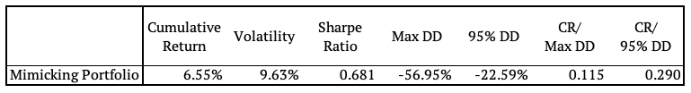
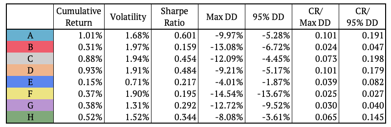
Secondly, we provide the risk & return table for both portfolios. The match of the factor portfolio meets our expectations, as it also matches the volatility and drawdowns well.
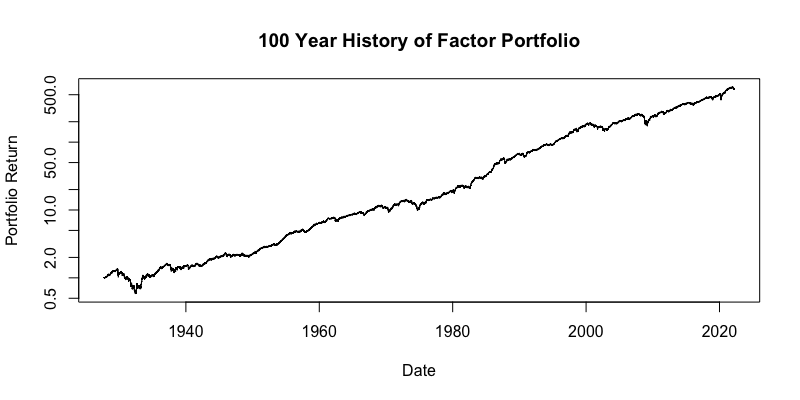
Now that we matched the AOR ETF, we can analyze the factor portfolio with the 100-year history. The figure below uses a log 10 y-axis. This is a chart depicting the hypothetical history of AOR US ETF going 100 years back into the past with daily data:
Market & Inflation
After obtaining the 100-year history of factor-matched AOR ETF, we can look at its performance during the combination of bull/bear markets and high/low inflation.
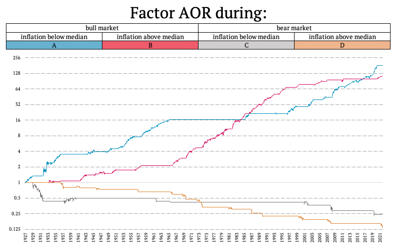
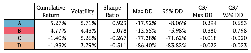
Pretty much as expected, the performance of a Balanced portfolio was mainly driven by equities throughout the entire history. Bull markets meant high returns for a balanced portfolio and, vice versa, bear markets meant low and negative returns. Inflation didn’t particularly influence these results.
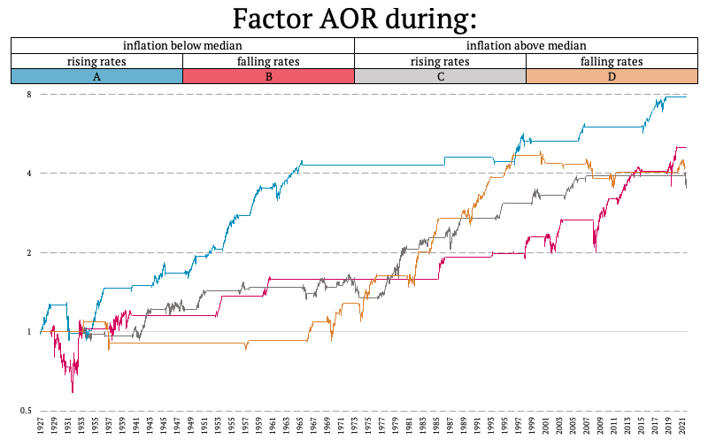
Nextly, let’s look at the performance of factor portfolio during high/low inflation and rising/falling rates.
Inflation & Rates
The performance of the factor AOR portfolio was positive during all of the combinations. The highest Sharpe ratio was achieved during low inflation periods with rising interest rates. On the other hand, looking at the risk side – maximum drawdown and volatility, the balanced portfolio performed worst during low inflation periods with falling interest rates.
The results are not so clear in this case. As we may observe, some pretty harsh drawdowns have historically occurred when rates were already declining and inflation was below median, which may be counterintuitive. However, as we explained in our previous article, this makes sense – because central banks usually already start cutting rates before the worst happens in the stock market and also inflation may already fall below its median before the bottom of the equity drawdown forms.
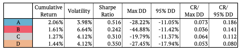
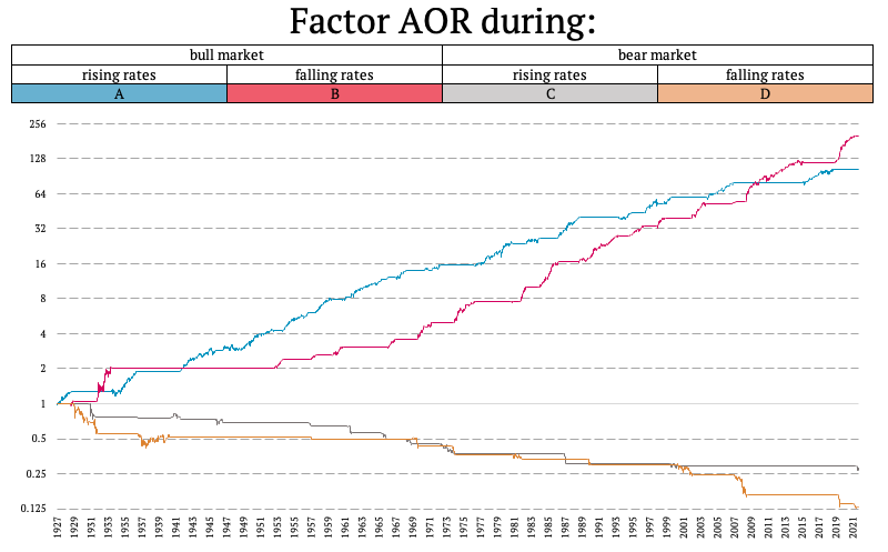
Market & Rates
Looking at the performance of the factor portfolio during the combinations of bull/bear market and rising/falling interest rates, the conclusion is very similar to the section above – where we analyzed Market & Inflation states. The results are mostly driven by equities, i.e. the performance is great in bull markets and bad in bear markets. We can also observe that the rise/ fall of interest rates doesn’t have any notable effect on the performance of the balanced portfolio during either a bull or a bear market.
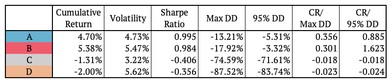
Market & Inflation & Rates
In addition to the double combinations, we also examined the performance of the factor portfolio during the combinations of the bull/bear market, low/high inflation, and rising/falling rates together. The following figure shows the portfolio’s performance.
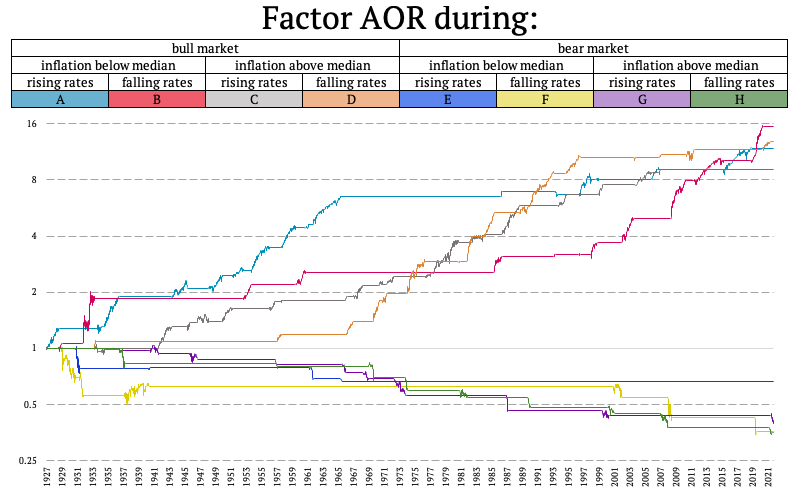
Once again, the results are naturally mainly driven by the state of the stock market. Bull is great Bear is poor. But, what is perhaps more interesting, is distinguishing among various states (of inflation and rates) in a bull market and then in a bear market.
We may observe that the highest Sharpe ratio has been achieved in the market cycle of high inflation and falling interest rates. On the other hand, the smallest Sharpe ratio (mainly due to highest volatility) appeared to happen over periods of low inflation and declining interest rates. These often seem to be the phases near market recessions (e.g. a recovery right after it) so the volatility is still elevated and this may dampen the Sharpe ratios.
A similar qualitative result may be observed for the bear market. Volatility is highest and returns are lowest again over periods of low inflation and already declining interest rates.
Trend-Following over 100 Years of different Market Cycles
We will now perform the same analysis of different historical market states for a Trend-Following strategy. At Quantpedia we were able to recreate a 100-year daily history for a Trend-Following strategy, that pretty well represents CTAs or trend-followers even nowadays. We described our methodology in detail in our article about 100 years of multi asset Trend-Following.
Market & Inflation
Similarly to AOR ETF let’s firstly look at the performance of multi-asset trend-following strategy (a.k.a. “Trend Factor”) during the combination of bull/bear markets and high/low inflation.
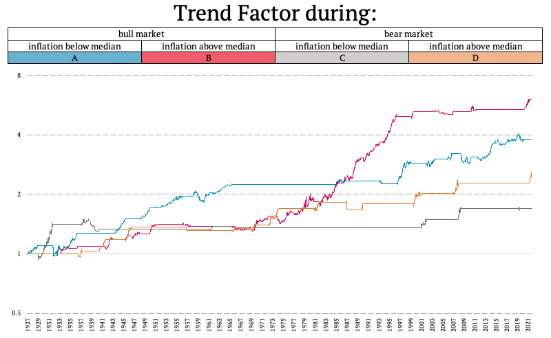
Now this is where the things start getting more interesting. The highest Sharpe ratio of a Trend-Following strategy has been achieved over a period of a bull market + inflation above median. But why? One possible explanation that fits may be, that the biggest trends are present in a final bull phase when markets peak and inflation is running hot.
On the other hand, the lowest Calmar and Sharpe ratio has been recorded over a period of a bear market + inflation below median. A possible hypothesis why this is so may be, that these are the periods where markets usually start to reverse (e.g. a final stage of a bear market, where inflation is already low again) and Trend-Followers obviously don’t like reversals.
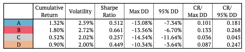
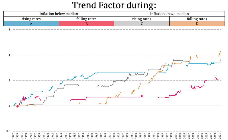
Secondly, let’s look at the performance of the strategy during high/low inflation and rising/falling rates.
Inflation & Rates
The performance of the strategy was positive during all of the combinations. However, the worst performance was achieved during low inflation and falling rates. Also, looking at the risk side – maximum drawdown and volatility, the portfolio performed worst during the combination of these periods.
This may be attributed to this phase again probably corresponding to a period of market reversals. When rates fall and inflation is (already) low, this usually happens e.g. when bear markets peak. Afterwards typically strong reversals do occur. And, as already mentioned, market reversals are periods when trend-followers suffer the most.
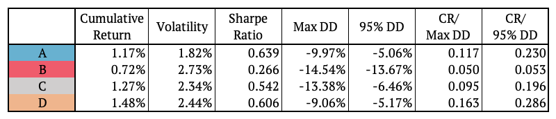
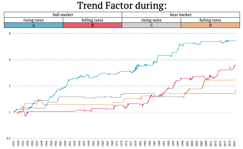
Market & Rates
Looking at the performance of a Trend-Following strategy during the combinations of bull/bear market and rising/falling interest rates, the conclusion is somewhat similar to an analysis of Market & Inflation states. The highest Calmar and Sharpe ratio were obtained over periods of bull markets and (paradoxically) rising interest rates.
Why rising and not falling rates? Well, it seems that the biggest trends (and the hottest economy) occur in bull markets when central banks already start raising the rates. Bull markets with falling rates seem to be the occasions during which the economy (and assets) still not perform strong enough for the FED to start cooling down the markets (and raising the rates).
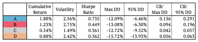
Market & Inflation & Rates
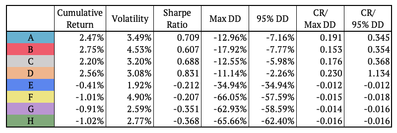
In addition to the double combinations, we also examined the performance of the Trend-Following during the combinations of the bull/bear market, low/high inflation, and rising/falling rates together. The following figure shows the portfolio’s performance.
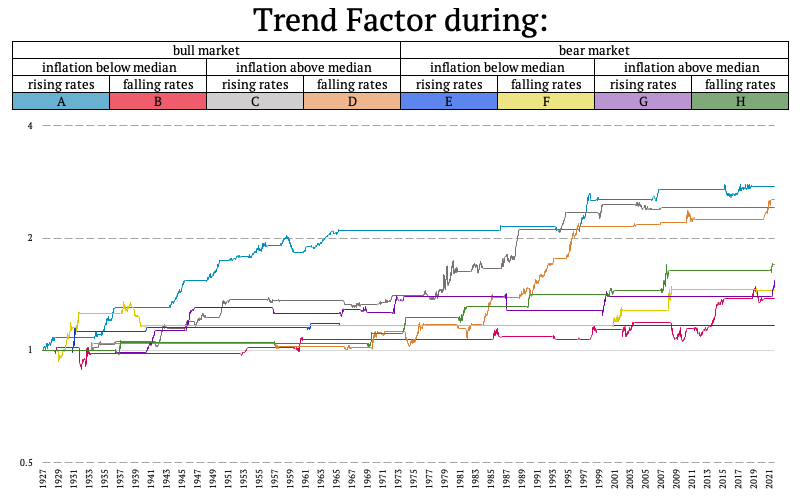
Here the relations are a bit more complex. We can for example point out to one of the more obvious explanation of depicted combinations – bull market + inflation above median + falling rates. This is the state we’ve been in quite recently, more specifically until the beginning of 2022. And this was a very strong period for Trend-Followers. Inflation has been already running high, rates were still supportive and stock markets have been peaking. Based on these quite strong trends, Trend-Followers recorded strong gains.
Conclusion and Coming Up Next
In this article we quantified the exact risk and return characteristics of a Balanced portfolio and a Trend-Following strategy over various market states during past 100 years of a market history. We examined how these portfolios perform when rates are rising or falling, what happens when inflation is above or below its median and how are these strategies affected by bull or bear markets in equities.
The analysis was based on already knowing with hindsight when the bull/bear market, high/low inflation and rising/falling interest rates already happened. This is particularly useful for anyone who has a firm view on where we are currently in the market state. If you get this view right, you can then position yourself with your asset allocation so that you benefit the most out of this state.
In the upcoming series of articles, we will take a closer look at an out-of-sample market cycle analysis. We will firstly aim to assess what market state are we currently in (and also historically) based only on the data points available up to that point in time. We will then also analyze in detail how do different assets perform going forward from this point. Stay tuned!
Author:
Daniela Hanicova, Quant Analyst, Quantpedia
Are you looking for more strategies to read about? Sign up for our newsletter or visit our Blog or Screener.
Do you want to learn more about Quantpedia Premium service? Check how Quantpedia works, our mission and Premium pricing offer.
Do you want to learn more about Quantpedia Pro service? Check its description, watch videos, review reporting capabilities and visit our pricing offer.
Do you want algorithmic access to the full Quantpedia database via the API? Subscribe to Quantpedia Pro, ask for an API key, and explore the in/out-of-sample statistics, source academic papers, and code snippets — ideal for quantitative research, systematic trading workflows, and AI model training.
Are you looking for historical data or backtesting platforms? Check our list of Algo Trading Discounts.
Or follow us on:
Facebook Group, Facebook Page, Telegram, Twitter, Linkedin, Medium or Youtube
Share onLinkedInTwitterFacebookRefer to a friend


