Avoid Equity Bear Markets with a Market Timing Strategy – Part 2
In this second installment in a series of three articles, we will continue with our goal to construct a market timing strategy that would sidestep the equity market during bear markets. A few days ago, we started with price-based market timing strategies. Today, we will focus on macroeconomic indicators and predictors derived from the movements in the commodity markets.
Market Timing Using Trend and Macroeconomic Indicators
In our search for reliable macroeconomic indicators that would improve our market-timing model, we came upon a blog by Philosophical Economics (2016). Likewise, they attempt to construct a market timing strategy that would switch from equities (the S&P 500) into cash (Treasury bills) before each recession and from cash back into equities once the recession is over. They start with market timing based on the SMA rule and face the exact issue as we do, i. e., on how to increase the strategy’s risk-adjusted return.
Conventional Macroeconomic Indicators
Philosophical Economics (2016) suggest that a natural way to enhance the strategy is to teach it to differentiate between situations where the fundamentals make the recession likely and situations where the fundamentals make the recession unlikely. Put differently, they propose a model that would stay invested in equities even if the MA signal is negative, but the macroeconomic environment is favorable. To quantify the U.S. macroeconomic image, they consider Real Retail Sales Growth (RSALES) and Industrial Production Growth (INDPROD) as they represent reliable indicators of the health of the two fundamental segments of the overall economy: consumption and production.
Their results show that when these macroeconomic signals are used with the MA rule separately, in both cases, the strategy’s risk-adjusted return improves, albeit the improvement is more substantial with RSALES. However, the best result emerges when both macro signals are used jointly, i.e., a strategy that stays invested in equities when the MA signal is positive or both RSALES and INDPROD signals are jointly positive.
Building upon their findings, we aim to improve our Naive strategy by adding RSALES and INDPROD signals and achieve results similar to Philosophical Economics (2016). To this end, we source RSALES and INDPROD data series from the FRED database, which is our primary source of macroeconomic data. When the obtained data don’t cover our entire sample period, we use the closest available proxy in the analysis.
We construct the trading signals for variables RSALES and INDPROD as follows:
- RSALES buys or stays long the MKT if Real Retail Sales Growth (YoY) in the prior month t-1 is positive,
- INDPROD buys or stays long the MKT if Industrial Production Growth (YoY) in the prior month t-1 is positive.
Note that when monthly economic numbers are published, they’re published for the prior month. Therefore, our macroeconomic signals use the previous month’s economic numbers, not the current month’s, which are unavailable. Our goal is that macro signals will keep us invested in the market when the economy is strong, regardless of the minor price fluctuations of MKT. That means our strategies switch off the stock market only if both trend and macro signals turn negative. However, only a positive trend signal can force us to return back to the stock market, a positive macro signal alone is not enough. We apply this condition to all our strategies that use macroeconomic trading signals.
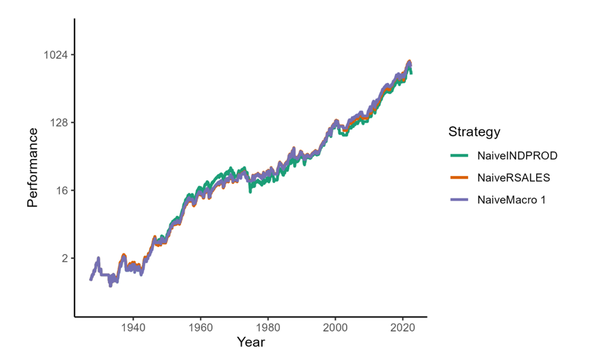
We add RSALES and INDPROD signals to our Naive strategy separately as well as jointly to form three strategies following Philosophical Economics (2016). NaiveINDPROD stays long the MKT if the Naive trading signal is positive or the INDPROD signal is positive. NaiveRSALES stays long the MKT if the Naive trading signal is positive or the RSALES signal is positive. NaiveMacro 1 stays long the MKT if the Naive trading signal is positive or INDPROD and RSALES signals are jointly positive. Otherwise, strategies switch out of the stock market.
Table 2 displays that all three strategies performed similarly, with NaiveRSALES notching the highest return of 7.16% p.a. and NaiveMacro 1 exhibiting the highest Sharpe ratio of 0.51. Our results from Table 2 indicate that adding macro signals to the Naive strategy significantly improves its return but at the cost of higher volatility and drawdowns, resulting in lower risk-adjusted returns. We can observe the performance of our strategies in Figure 2 as well, showing that their equity curves move jointly almost the entire sample period, except for the NaiveINDPROD in 1960-1990 and the early 2000s. Overall, our results are consistent with those of Philosophical Economics (2016) and confirmed that some macroeconomic indicators contain valuable information about future stock market returns, so we continued our search for novel and reliable macroeconomic indicators that could further improve our model.
Table 2: Performance summary of market timing strategies by Philosophical Economics for the period from April 1927 to June 2022. MKT and Naive are added as benchmarks. The best-performing strategy is shaded.
| Strategy | Ann Return | Ann Volatility | Max DD | Sharpe Ratio | Calmar Ratio | Time In | Corr Naive |
| NaiveINDPROD | 6.86% | 14.66% | -58.00% | 0.47 | 0.12 | 88.19% | 0.820 |
| NaiveRSALES | 7.16% | 14.42% | -58.00% | 0.50 | 0.12 | 85.04% | 0.833 |
| NaiveMacro 1 | 7.13% | 14.08% | -58.00% | 0.51 | 0.12 | 82.76% | 0.853 |
| MKT | 6.56% | 18.55% | -84.63% | 0.35 | 0.08 | 100.00% | 0.647 |
| Naive | 6.30% | 12.06% | -54.97% | 0.52 | 0.11 | 67.54% | 1.000 |
Figure 2: Performance chart of market timing strategies by Philosophical Economics for the period from April 1927 to June 2022.
Commodity Indicators
Demand for industrial commodities, e.g., copper, oil, or lumber, relative to the demand for safe-haven assets such as gold, has traditionally been seen as a leading indicator of global economic health. Rising demand for industrial commodities relative to gold indicates that the economy is running at full steam, i.e., expansion, implying higher returns for the stock market. Conversely, falling demand for industrial commodities relative to gold points to a slowdown in production, suggesting that the economy may be slipping into recession, which in turn leads to lower stock market returns.
In his paper, Gayed (2015) showed that the relative performance of lumber to gold contains a significant predictive power that can be utilized in market timing. He explains that when lumber outperforms gold, equities tend to exhibit an upward bias and have lower volatility, making it favorable to take more risk in a portfolio. As gold outperforms lumber, the opposite tends to be true, whereby moving into low-risk assets increases overall return and lowers volatility. His trading strategy, which switches on a weekly basis from Treasuries to stocks when lumber outperforms gold and from stocks back to Treasuries when gold outperforms lumber, improves both absolute and risk-adjusted return metrics relative to simply buying and holding an equity index. In a similar study, Fang (2020) examined the ability of ten gold price ratios, defined as the dollar price of gold to the price of an individual asset, to predict aggregate stock returns. He found that seven out of ten gold price ratios significantly predict stock returns. Among these ratios, the gold-to-oil ratio is the most powerful return predictor, whose information does not overlap with the information contained in traditional predictors and other gold price ratios.
Building upon these findings, we construct three trading signals based on the performance of an industrial commodity versus gold as follows:
- COPGLD buys or stays long the MKT if the copper three-month performance is greater or equal to the gold three-month performance,
- OILGLD buys or stays long the MKT if the oil three-month performance is greater or equal to the gold three-month performance,
- LUMGLD buys or stays long the MKT if the lumber three-month performance is greater or equal to the gold three-month performance.
Note that although these are macroeconomic signals, they are calculated from commodity prices, which are available at any time and don’t have to be lagged by one month as our other macroeconomic signals. We add the constructed trading signals to our Naive strategy and obtain three commodity strategies. NaiveCOPGLD stays long the MKT if the Naive trading signal is positive or the COPGLD signal is positive. NaiveOILGLD stays long the MKT if the Naive trading signal is positive or the OILGLD signal is positive. NaiveLUMGLD stays long the MKT if the Naive trading signal is positive or the LUMGLD signal is positive. Otherwise, strategies switch out of the stock market.
We can observe the performance of our commodity strategies in Table 3. The best-performing commodity strategy in terms of absolute and risk-adjusted returns, NaiveCOPGLD, exhibits an annual return of 6.97% and a Sharpe ratio of 0.54, which is greater than that of Naive. NaiveLUMGLD, on the other hand, displays the lowest annual volatility of 12.84% and the most favorable maximal drawdown of -54.97%. Although some commodity strategies managed slightly improve Naive’s risk-adjusted returns, they suffer substantial drawdowns, which are unacceptable in a market timing strategy.
Unemployment and Dividend Indicators
In our next course of action, we return to the NaiveMacro 1 strategy proposed by Philosophical Economics (2016) and try to improve it by introducing new macroeconomic trading signals. To this end, we source the U.S. unemployment rate data series from FRED and S&P Composite dividends series from Robert Shiller’s website. We construct the trading signals for our new macroeconomic variables as follows:
- UNRATE buys or stays long the MKT if the U.S. unemployment rate by the Bureau of Labor Statistics in the prior month t-1 falls or remains the same compared to month t-2,
- DIVIDEND buys or stays long the MKT if real S&P Composite dividends per share in the prior month t-1 increase compared to the month t-2.
Our macroeconomic signals UNRATE and DIVIDEND are inspired by Philosophical Economics (2016), which uses employment growth and real S&P 500 EPS growth in their market timing strategy. We prefer to use the UNRATE signal instead of employment growth as it has a longer data series, making it more reliable. Additionally, it is a more closely watched indicator by investors. Similarly, we prefer using the DIVIDEND signal instead of real S&P 500 EPS growth. Dividends represent an actual payout to an investor for holding the shares, making them a more tangible and reliable indicator of economic performance.
In their blog, Philosophical Economics (2016) explain that although both employment growth and real S&P 500 EPS growth are lagging indicators of recession, they can work well when used jointly with a trend signal. It is because their main role is to keep strategy invested in the stock market when the economy is strong. Their study shows that both indicators improve market timing results by SMA rule but not as much as INDPROD or RSALES. Note that their blog uses employment growth and real S&P 500 EPS growth with the MA rule only separately. We fill this gap and use our UNRATE and DIVIDEND signals with Naive separately as well as jointly with all our other macro signals.
Our NaiveUNRATE strategy stays long the MKT if the Naive trading signal is positive or the UNRATE signal is positive. NaiveDIVIDEND stays long the MKT if the Naive trading signal is positive or the DIVIDEND signal is positive. NaiveMacro 2 stays long the MKT if the Naive trading signal is positive or INDPROD, RSALES, UNRATE, and DIVIDEND signals are jointly positive. TrendMacro 1 stays long the MKT if the Trend trading signal is positive or INDPROD, RSALES, UNRATE, and DIVIDEND signals are jointly positive. Otherwise, strategies switch out of the stock market.
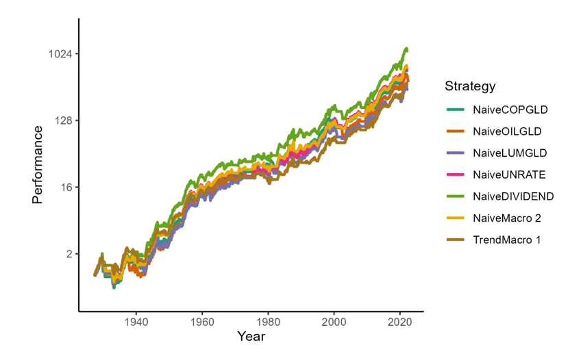
Table 3 reports the results. The introduction of UNRATE and DIVIDEND signals improved our market timing results as our new strategies did substantially better compared to commodity trading strategies as well as those proposed by Philosophical Economics (2016). NaiveDIVIDEND displays the highest annual return of 7.64% so far and the highest Sharpe ratio of 0.57. However, this exceptional performance is at the cost of a sharp maximal drawdown of -59.10%. NaiveUNRATE and NaiveMacro 2 show similar results, although NaiveMacro 2 exhibits a little lower volatility as it relies on multiple macroeconomic trading signals. Our final macro strategy, TrendMacro 1, does exactly what a solid market timing strategy should do. In the introduction, we mentioned that the ultimate goal of market timing is to realize market returns at lower volatility and milder drawdowns. Our strategy exhibits an annual return of 6.45%, close to that of MKT while cutting the volatility by a third to 11.93% p.a. and maximal drawdown by half to -42.87%. Nevertheless, its Sharpe ratio at 0.54 is slightly lower when compared with some of our other macroeconomic strategies.
Although TrendMacro 1 shows superior results, there is still room for improvement. Figure 3 shows that strategy (muted brown line) correctly exits MKT during bear markets. It is because the strategy switches out of the stock market after the Trend signal turns negative, assuming that at least one of its macro signals is also negative. However, by the time that happens, it can cumulate a significant amount of losses. For example, during the Wall Street Crash of 1929, the strategy exits the stock market for the first time when it is already down nearly 25% from its peak. Naturally, a trading signal that could switch the strategy off the stock market before the bear market even starts can substantially improve its performance. The good news is that academic literature knows one reliable indicator that can herald a looming bear market, which is the yield curve.
Table 3: Performance summary of macroeconomic market timing strategies for the period from April 1927 to June 2022. MKT and Naive are added as benchmarks. The best-performing strategy is shaded.
| Strategy | Ann Return | Ann Volatility | Max DD | Sharpe Ratio | Calmar Ratio | Time In | Corr Naive |
| NaiveCOPGLD | 6.97% | 12.91% | -60.20% | 0.54 | 0.12 | 74.93% | 0.931 |
| NaiveOILGLD | 6.57% | 13.67% | -60.20% | 0.48 | 0.11 | 79.93% | 0.880 |
| NaiveLUMGLD | 6.34% | 12.84% | -54.97% | 0.49 | 0.12 | 73.44% | 0.939 |
| NaiveUNRATE | 7.01% | 12.98% | -54.97% | 0.54 | 0.13 | 75.15% | 0.926 |
| NaiveDIVIDEND | 7.64% | 13.51% | -59.10% | 0.57 | 0.13 | 79.00% | 0.888 |
| NaiveMacro 2 | 7.07% | 12.45% | -54.97% | 0.57 | 0.13 | 70.78% | 0.966 |
| TrendMacro 1 | 6.45% | 11.93% | -42.87% | 0.54 | 0.15 | 66.14% | 0.937 |
| MKT | 6.56% | 18.55% | -84.63% | 0.35 | 0.08 | 100.00% | 0.647 |
| Naive | 6.30% | 12.06% | -54.97% | 0.52 | 0.11 | 67.54% | 1.000 |
Figure 3: Performance chart of macroeconomic market timing strategies for the period from April 1927 to June 2022.
We will end the article at this point and continue on Friday. The last part of this series will investigate yield-based recession predictors and tries to wrap all ideas into one coherent framework for the final market timing strategy. Therefore, say tuned for our continuation in part 3 – Market Timing Using Yield Curve.
Author:
Ladislav Durian, Quant Analyst, Quantpedia
Are you looking for more strategies to read about? Sign up for our newsletter or visit our Blog or Screener.
Do you want to learn more about Quantpedia Premium service? Check how Quantpedia works, our mission and Premium pricing offer.
Do you want to learn more about Quantpedia Pro service? Check its description, watch videos, review reporting capabilities and visit our pricing offer.
Are you looking for historical data or backtesting platforms? Check our list of Algo Trading Discounts.
Would you like free access to our services? Then, open an account with Lightspeed and enjoy one year of Quantpedia Premium at no cost.
Or follow us on:
Facebook Group, Facebook Page, Twitter, Linkedin, Medium or Youtube
Share onLinkedInTwitterFacebookRefer to a friend