Avoid Equity Bear Markets with a Market Timing Strategy – Part 3
In the last third installment, we will finish exploring the world of market timing strategies (see parts 1 & 2). We will focus on yield curve predictors and incorporate all three ideas (price-based, macro-economic, and yield curve predictors) into one final trading strategy that yields an annual return above that of the stock market while doubling its Sharpe ratio and reducing maximal drawdown by two thirds.
Market Timing Using Yield Curve
The term yield curve refers to the relationship between the short- and long-term interest rates of fixed-income securities issued by the U.S. Treasury. Under normal circumstances, the yield curve slopes upwards since debt with longer maturities typically carries higher interest rates than nearer-term ones. An inverted yield curve occurs when short-term interest rates exceed long-term rates. From an economic perspective, an inverted yield curve is noteworthy and uncommon because it suggests that the near-term is riskier than the long-term.
The slope of the yield curve is influenced by monetary policy and investor expectations. Rising short-term rates due to expansionary monetary policy could lead to a slowdown in economic activity and demand for credit as borrowing becomes more expensive. At the same time, slowing activity may result in lower inflation, increasing the likelihood of a future monetary policy easing. This expectation of future rate cuts can lead to an inversion of the yield curve as investors anticipate lower interest rates in the future. This scenario explains the observed correlation between the yield curve and recessions.
Extensive literature has developed in support of the yield curve as a reliable predictor of recessions and equity bear markets. Estrella and Mishkin (1996) analyzed the predictive power of the yield curve to forecast recessions in the timespan from the first quarter of 1960 to the first quarter of 1995. To this end, they construct a probit model that translates the steepness of the yield curve at the present time into a likelihood of a recession one, two, four, or six quarters ahead. They measure the steepness by the spread between the ten-year Treasury rate and the three-month Treasury rate as this combination of rates is accurate and robust in predicting U.S. recessions over long periods. They compared its forecasting performance with other indicators such as the New York Stock Exchange stock price index, the Commerce Department’s index of leading economic indicators, and the Stock-Watson index. The yield curve outperformed all indicators in predicting recessions two or more quarters ahead, with no wrong signal and the best performance four quarters ahead. Therefore, they conclude that the Treasury spread is useful in macroeconomic prediction, particularly with a longer lead.
Figure 4: Probability of U.S. recession four quarters ahead predicted by the yield curve or NYSE stock price index from Q1 1971 to Q1 1995. Shaded areas indicate periods designated as national recessions by the NBER.
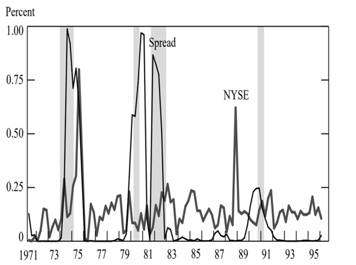
Source: Estrella and Mishkin (1996)
Based on the findings of Estrella and Mishkin (1996), Resnick and Shoesmith (2002) extend the probit model to forecast equity bear markets in the U.S. For the timespan from January 1971 through December 1999, they use the probit model with the spread between the 10-year and 3- month Treasuries as the explanatory variable. Their model forecasts a bear market one and two months in advance, with one-month results being preferable. A simulation using the out-of-sample time series of probabilities for a stock bear market showed that using a 50% probability threshold, an investor could outperform the S&P 500. While the buy-and-hold strategy on the S&P 500 would have gained a compounded return of 14.17% annually, a strategy in which the investor switched from T-bills to the S&P 500 if the probability of a bear market one month later was less than 50% and vice versa gained annually 16.46% and hence outperforming the benchmark by 229 basis points.
Figure 5: S&P 500 and probability of a bear stock market from January 1971 to December 1999. Shaded regions indicate five S&P 500 bear markets in this period.
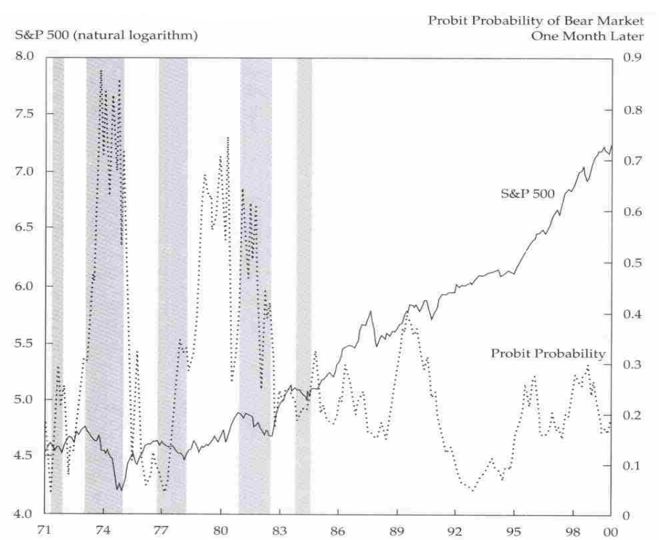
Source: Resnick and Shoesmith (2002)
Building upon the superior predictive results of the yield curve for the U.S. recessions and equity bear markets in the academic literature, we first add the yield curve signal to our Naive and Trend strategies. Our trading signal for the yield curve is as follows:
- YC buys or stays long the MKT if the 10-year Treasury yield is greater than the 3-month Treasury yield.
Accordingly, NaiveYC buys or stays long MKT if the Naive trading signal and YC signal are jointly positive. TrendYC buys or stays long MKT if the Trend trading signal and YC signal are jointly positive. Otherwise, strategies switch out of the stock market. In both cases, incorporating the YC signal into the strategy boosted the risk-adjusted returns, as indicated in Table 4. Naive’s Sharpe ratio grew from 0.52 to 0.55 and the Calmar ratio from 0.11 to 0.15. The Trend’s improvement was less pronounced as its Sharpe ratio rose from 0.51 to 0.54 and the Calmar ratio from 0.14 to 0.15. Note that both strategies exhibit results similar to TrendMacro 1 using just two trading signals, highlighting the superior predictive power of the yield curve.
Next, we include the YC signal among macroeconomic indicators in our NaiveMacro 2 and TrendMacro 1 strategies to obtain their two enhanced versions. NaiveMacro 3 stays long MKT if the Naive trading signal is positive or INDPROD, RSALES, UNRATE, DIVIDEND, and YC signals are jointly positive. TrendMacro 2 stays long MKT if the Trend trading signal is positive or INDPROD, RSALES, UNRATE, DIVIDEND, and YC signals are jointly positive. Otherwise, strategies switch out of the stock market.
The resultant strategies NaiveMacro 3 and TrendMacro 2 in Table 4 show the exact results as their counterparts NaiveMacro 2 and TrendMacro 1 in Table 3 since they are equivalent. In this case, including the YC signal did not make any difference. It is because the only way YC can affect the strategy’s performance is when it turns negative before any other macroeconomic signal under the assumption that the trend signal is also negative. Note that our strategies switch off the stock market only if both trend and macro signals turn negative. However, YC mostly turns negative even before the trend indicators, forecasting an impending bear market, and then turns positive once the bear market starts (even before trend indicators turn negative) as the central bank cuts rates. It is because the yield curve is a leading indicator of a bear market, while our other macroeconomic indicators are lagging indicators.
Figure 6: Spread between the 10-year Treasury yield and the 3-month Treasury yield from April 1927 to June 2022. Shaded areas indicate bear markets in this period.
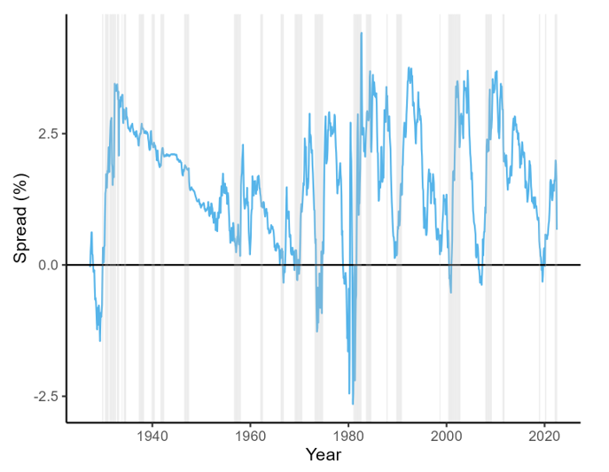
Figure 6 shows that the Treasury spread turned negative before every major bear market during our sample period as did before the Wall Street Crash of 1929, the 1973–1974 stock market crash, the Early 1980s recession, the Dot-com bubble in the early 2000s, the 2007–2008 financial crisis, and the 2020 stock market crash.
The Final Strategy
To fully utilize the YC’s ability to forecast the bear market before it even starts, we drop it from our macroeconomic predictors and use its signal jointly with Trend instead.
| The trading rule for our final strategy is as follows: TrendYCMacro stays long MKT if the Trend and YC trading signals are both positive or INDPROD, RSALES, and DIVIDEND signals are jointly positive. Otherwise, the strategy switches out of the stock market. |
Note that we dropped UNRATE from our macroeconomic predictions as well since it produced many false signals, dragging down the strategy’s performance. In this setup, the strategy exits the stock market not only when the Trend signal turns negative but already when YC turns negative, assuming that at least one of the macro signals is also negative. This allows the strategy to avoid the initial declines in bear markets because the YC would switch it off even before the bear market starts and therefore doesn’t have to wait for the Trend to turn negative. If accidentally, Trend or YC generates a false negative signal, the strategy would stay invested in the stock market as long as the economy is strong, i.e., INDPROD, RSALES, and DIVIDEND signals are jointly positive.
Table 4 demonstrates the impressive performance of TrendYCMacro, with an annual return of 7.05% that surpasses both MKT and Naive. The maximum drawdown of -25.13% is the lowest among all strategies, which is only a third of that of MKT and half of Naive. Additionally, with an annual volatility of 11.83%, TrendYCMacro has the highest risk-adjusted performance, as indicated by its highest Sharpe ratio of 0.60 and Calmar ratio of 0.28 among all our strategies. These results proved that TrendYCMacro outperformed its benchmarks, MKT and Naive, across all performance metrics. A visual comparison of TrendYCMacro with other market timing strategies based on the YC signal can be found in Figure 7.
Table 4: Performance summary of market timing strategies with YC signal for the period from April 1927 to June 2022. MKT and Naive are added as benchmarks. The best-performing strategy is shaded.
| Strategy | Ann Return | Ann Volatility | Max DD | Sharpe Ratio | Calmar Ratio | Time In | Corr Naive |
| NaiveYC | 6.25% | 11.38% | -41.28% | 0.55 | 0.15 | 62.73% | 0.943 |
| TrendYC | 5.92% | 10.94% | -40.37% | 0.54 | 0.15 | 58.62% | 0.905 |
| NaiveMacro 3 | 7.07% | 12.45% | -54.97% | 0.57 | 0.13 | 70.78% | 0.966 |
| TrendMacro 2 | 6.45% | 11.93% | -42.87% | 0.54 | 0.15 | 66.14% | 0.937 |
| TrendYCMacro | 7.05% | 11.83% | -25.13% | 0.60 | 0.28 | 65.70% | 0.839 |
| MKT | 6.56% | 18.55% | -84.63% | 0.35 | 0.08 | 100.00% | 0.647 |
| Naive | 6.30% | 12.06% | -54.97% | 0.52 | 0.11 | 67.54% | 1.000 |
Figure 7: Performance chart of market timing strategies with YC signal for the period from April 1927 to June 2022.
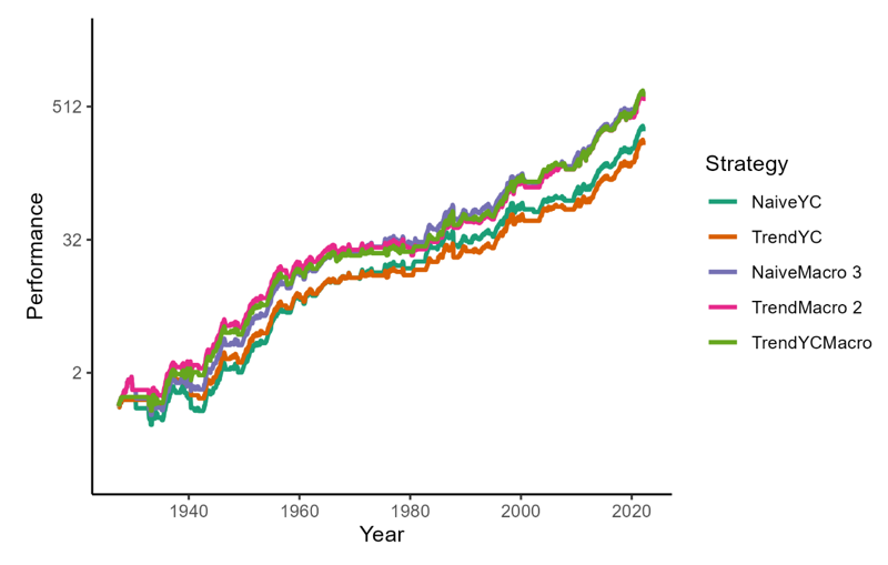
Figure 8 highlights the remarkable market timing results of our strategy, TrendYCMacro. During major bear markets, TrendYCMacro effectively exited the stock market, often prior to the start of the downturn. The most prominent example of this timing ability is its exit in December 1926, just before the onset of the Wall Street Crash of 1929. The YC signal also successfully turned the strategy off before other significant market crashes, including the 1973-1974 stock market crash, the Early 1980s recession, the Dot-com bubble, the 2007-2008 financial crisis, and the 2020 stock market crash.
Figure 8: Performance chart of TrendYCMacro strategy for the period from April 1927 to June 2022. Shaded areas indicate bear markets.
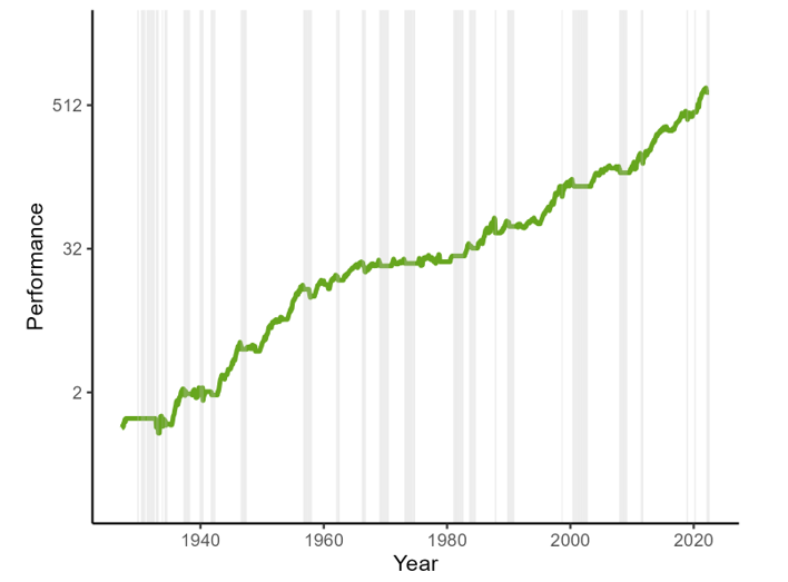
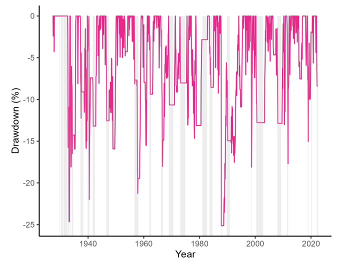
Figure 9 shows that our final market timing strategy has experienced a low level of volatility, with drawdowns rarely exceeding 15%, comparable to the stability offered by traditional bonds. And although TrendYCMacro suffered a maximum drawdown of -25.13% in October 1987 during Black Monday, it is worth noting that timing such an event with a monthly market timing strategy is inherently challenging.
Figure 9: Drawdown chart of TrendYCMacro strategy for the period from April 1927 to June 2022. Shaded areas indicate bear markets.
Conclusion
Our goal was to construct a market timing strategy that would reliably sidestep the equity market during bear markets and thereby reduce market volatility and boost risk-adjusted returns. In the first part of the paper, we attempted to time the market using price-based indicators, i.e., moving averages, volatility, skewness, RSI, and Rachev ratio. Among these indicators, only trading signals from the 200-day SMA, used in our Naive strategy, and an alternative performance metric Rachev ratio delivered satisfactory results, so we combined them to obtain a more diversified signal, Trend.
In the second part, inspired by Philosophical Economics (2016), we introduced macroeconomic trading signals to our Naive and Trend strategies with the aim of improving their risk-adjusted returns. Our set of macroeconomic indicators included conventional macroeconomic indicators, such as Real Retail Sales Growth and Industrial Production Growth, commodity indicators reflecting industrial commodity vs. gold performance, and finally, unemployment and dividend indicators. Our notion was that trading signals based on macroeconomic indicators would keep us invested in the market when the economy is strong, regardless of the stock market fluctuations, reducing unnecessary exits of our strategies. And while the commodity trading signals failed accurately predict bear markets, the inclusion of the conventional indicators, and unemployment and dividend indicators significantly improved absolute and risk-adjusted returns of our strategies. Our best-performing macroeconomic strategy, TrendMacro 1, which uses Trend signal as a trend indicator and INDPROD, RSALES, UNRATE, and DIVIDEND signals as macroeconomic indicators, reduced market volatility by a third and the maximal drawdown by half.
In the third part, we incorporated information from the yield curve, i.e., the yield spread between 10-year Treasuries and 3-month Treasuries, into our macroeconomic strategies as it is a recognized and reliable leading indicator of recessions and equity bear markets. Although adding a YC signal among the macroeconomic predictors did not lead to any improvement, the use of the YC jointly with trend signals boosted risk-adjusted returns and substantially reduced drawdowns. Our final strategy, TrendYCMacro, which stays long MKT if the Trend and YC trading signals are both positive or INDPROD, RSALES, and DIVIDEND signals are jointly positive, yields an annual return well above that of MKT while doubling its Sharpe ratio and reducing maximal drawdown by two thirds.
Author:
Ladislav Durian, Quant Analyst, Quantpedia
Are you looking for more strategies to read about? Sign up for our newsletter or visit our Blog or Screener.
Do you want to learn more about Quantpedia Premium service? Check how Quantpedia works, our mission and Premium pricing offer.
Do you want to learn more about Quantpedia Pro service? Check its description, watch videos, review reporting capabilities and visit our pricing offer.
Are you looking for historical data or backtesting platforms? Check our list of Algo Trading Discounts.
Would you like free access to our services? Then, open an account with Lightspeed and enjoy one year of Quantpedia Premium at no cost.
Or follow us on:
Facebook Group, Facebook Page, Twitter, Linkedin, Medium or Youtube
Share onLinkedInTwitterFacebookRefer to a friend