How Much Bitcoin Should We Allocate To the Portfolio?
Introduction
After years of waiting, the recent launch of spot Bitcoin ETFs marked a significant milestone in the cryptocurrency market, making Bitcoin even more accessible for investors. Spot ETFs provide a convenient and regulated way to gain exposure to Bitcoin without the need to hold the digital asset directly, potentially attracting a broader range of market participants. Many investors are waiting to see this change’s long-term impact on the cryptocurrency’s price while putting their faith in the potentially significant returns from Bitcoin within their investment portfolios. These events are taking place after two significant milestones in Bitcoin’s history – the introduction of BTC futures in 2017 and the launch of the BTC futures ETF (BITO) in 2021. While examining the whole history of Bitcoin may give the impression of a new super asset, we need to set realistic expectations. What have all these historical changes brought, and what lessons can we learn from similar occurrences involving other assets throughout history?
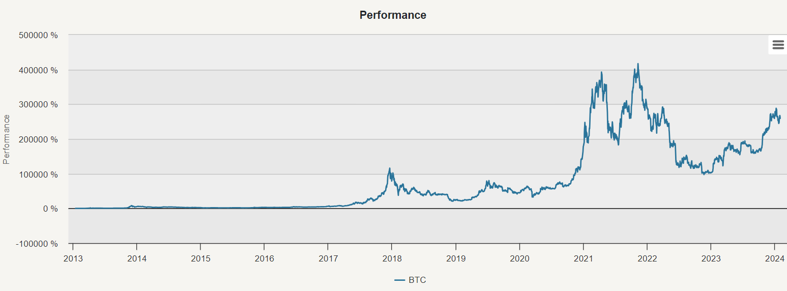
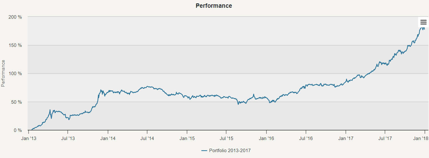
Examining the whole graph, covering the period from 2013 to 2023, it’s easy to get the impression that becoming a millionaire is within reach. The strategy to hold BTC between 2013 and 2023 exhibits a CAR (Compound Annual Return) of 103,77%. However, using the entire 11-year graph and extrapolating any long-term conclusions is misleading. From 2013 to 2017, cryptocurrencies were an obscure asset class known only to enthusiasts. This period represented a unique chapter in the evolution of digital currencies – when cryptocurrencies were still beginning, with limited mainstream recognition. It was a time of experimentation, with various cryptocurrencies emerging, often driven by passionate communities of supporters. Such a period is unlikely to happen again – it was a singular, once-in-a-lifetime occurrence. But what significant event reshaped the world of cryptocurrency in 2017?

Financialization
The introduction of futures trading on Bitcoin by the Chicago Board of Options Exchange (CBOE) on December 10, 2017, followed by the Chicago Mercantile Exchange (CME) on December 18, 2017, marked a milestone development in the cryptocurrency space. A liquid financial instrument became available legally for the first time in history, allowing funds and hedge funds to buy and sell Bitcoin in their portfolios without needing to open accounts in unregulated (and often very very shady) crypto exchanges. This event facilitated the financialization of cryptocurrency markets, a term describing how a market becomes integrated into the broader financial system and gains characteristics similar to traditional financial assets.
The financialization of cryptocurrency markets mirrors similar developments in emerging markets and commodities. Once considered obscure asset classes, emerging markets and commodities underwent a similar transformation. Initially, only specialized funds traded in these markets, but introducing indexes and ETFs in the mid-2000s made commodities more accessible to mainstream investors.
A similar path can be expected for cryptocurrencies. As cryptocurrencies continue to become more increasingly integrated into the global financial system and attract demand from institutional investors, they will undergo a process of financialization. This evolution will likely involve introducing more financial instruments, such as active ETFs and broad indexes, making cryptocurrencies more accessible to a broader investor base. However, it’s essential to approach this transformation with caution. Similar to commodities, past performance of cryptocurrencies may not accurately reflect future outcomes, especially as market dynamics shift with increased institutional involvement. Investors should be mindful of the changing landscape and adjust their strategies accordingly, looking at the history of Bitcoin in two different periods – pre-financialization and post-financialization.
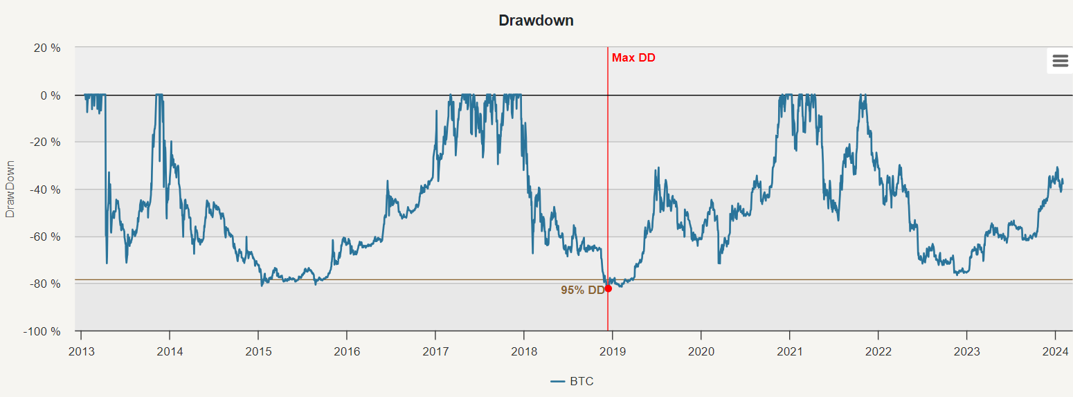
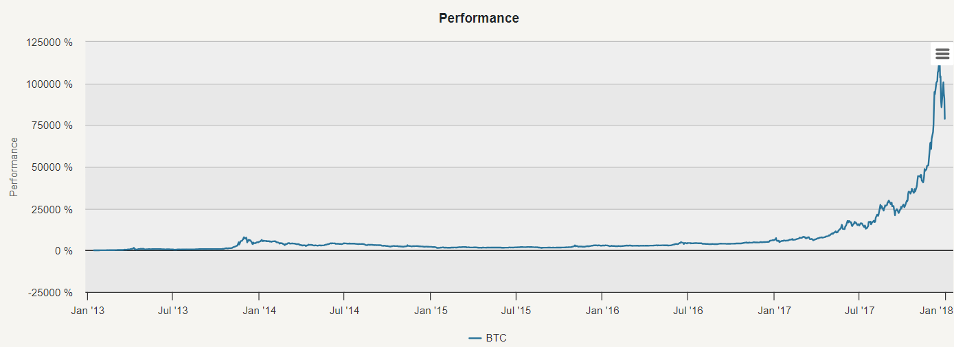
First, let’s look at the first period – until 2017. The cryptocurrency experienced extraordinary growth, with a remarkable compounded annual return of 283.33%. However, this period was also marked by significant volatility, with fluctuations in price reaching 95.83%. The maximum drawdown during this time was -81.15%. This pre-financialization period offered exceptional Bitcoin’s risk-return characteristics with a Sharpe ratio of 2.96 and Calmar ratio (CAR/MaxDD) of 3.49.

As we can see on the graph below, futures trading on Bitcoin was launched by the Chicago Board Options Exchange (CBOE) on December 10, 2017, followed closely by the Chicago Mercantile Exchange (CME) on December 18, 2017. Secondly, on October 19, 2021, another milestone was reached with the launch of the first Bitcoin futures exchange-traded fund (BITO). Introducing a Bitcoin futures ETF represented an important step towards mainstream acceptance of cryptocurrencies within traditional financial markets. Finally, on January 10, 2024, the launch of spot Bitcoin ETFs marked a significant milestone in the cryptocurrency market. Unlike futures-based ETFs like BITO, spot ETFs would directly hold Bitcoin, offering investors exposure to the actual cryptocurrency itself rather than futures contracts.
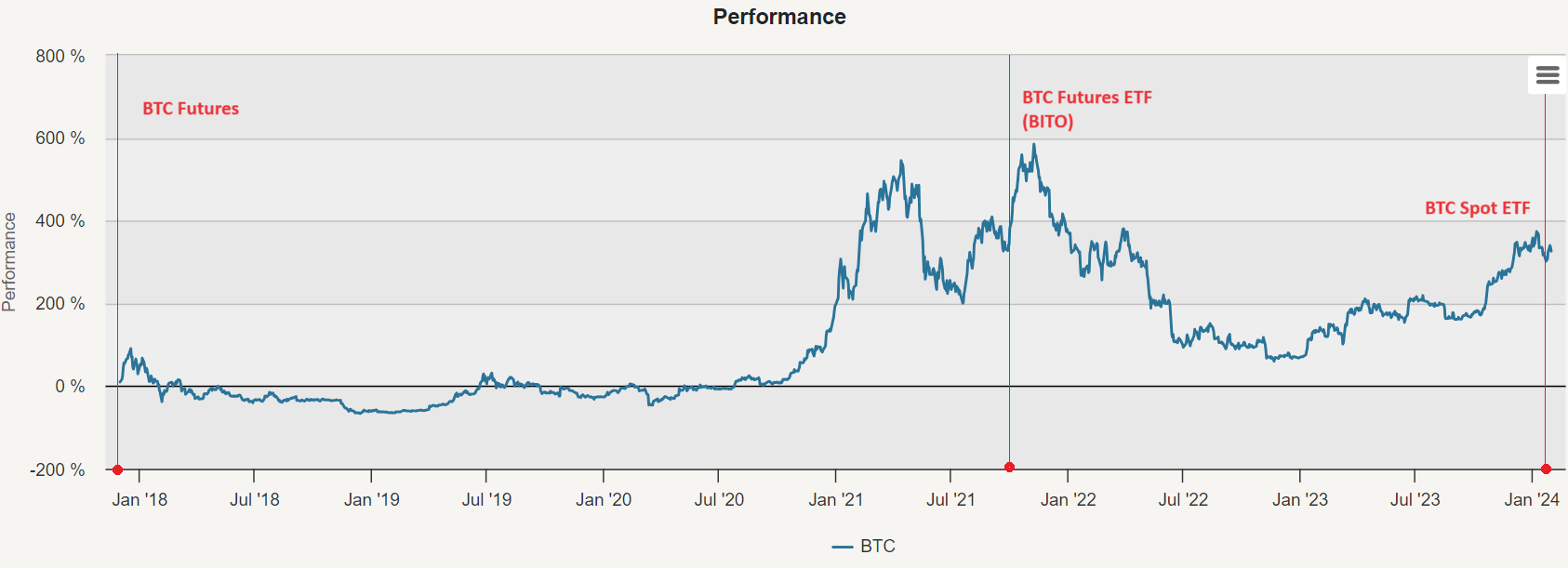

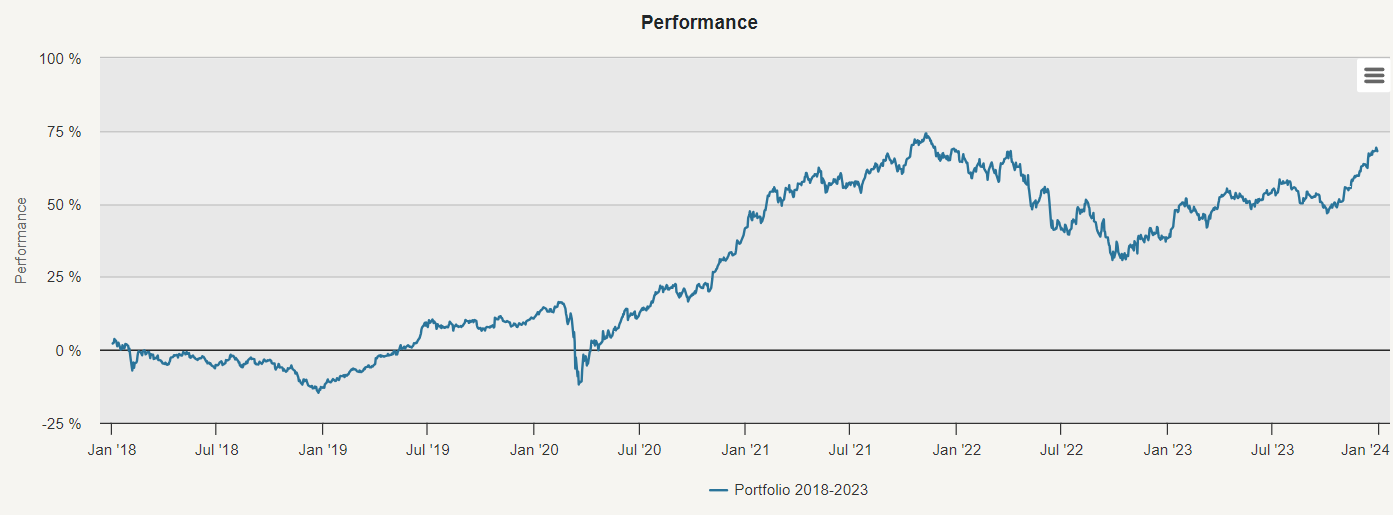
In contrast to the enormous rise experienced in Bitcoin’s earlier years, 2018 to 2023 presented a compounded annual Return of 21.95%. Volatility stayed high, though less than before, at 70.89%, showing Bitcoin might be getting steadier, but still with a significantly high maximum drawdown of -79.75%. Bitcoin’s risk-return ratios in the post-financialization period are nothing spectacular, with a Sharpe ratio of just 0.31 and a Calmar ratio of 0.28.
Naturally, questions arise: How much Bitcoin should we allocate to the portfolio?
Main Analysis
The main analysis examines a globally diversified portfolio across various asset classes, offering exposure to various geographic regions and investment instruments. The equally weighted portfolio consists of
- SPY (SPDR S&P 500 ETF)
- EEM (iShares MSCI Emerging Markets ETF)
- EFA (iShares MSCI EAFE ETF)
- IYR (iShares U.S. Real Estate ETF)
- IEF (iShares 7-10 Year Treasury Bond ETF)
- LQD (iShares iBoxx $ Investment Grade Corporate Bond ETF)
- HYG (iShares iBoxx $ High Yield Corporate Bond ETF)
- DBC (Invesco DB Commodity Index Tracking Fund)
- GLD (SPDR Gold Trust)
- and finally BTC (Bitcoin)
2013-2017
In our initial analysis, we examined an equally weighted portfolio over the period from 2013 to 2017. This allocation yielded a notable return of 22.86% alongside volatility of 11.76% and a maximum drawdown of -18.02%. Subsequently, we used the Portfolio Analysis to analyze correlations between different assets and Bitcoin, the Markowitz model to find the optimal portfolio that realizes the highest possible Sharpe ratio, and the Risk Parity for an alternative way to build a portfolio with a reduced concentration of the risk.

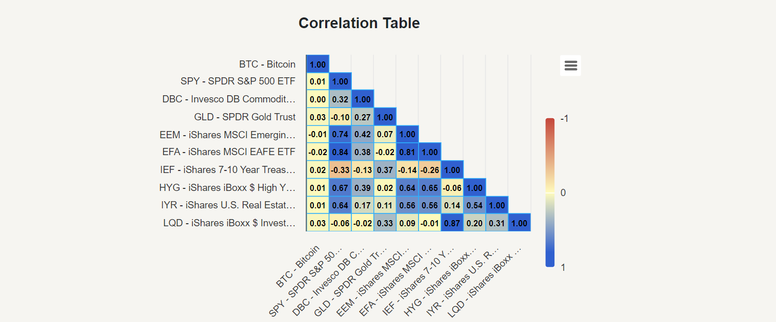
Correlation Table
Firstly, we looked into the Correlation Table to understand the relationship between Bitcoin and other assets. We found that the correlation of Bitcoin with other assets in the period of 2013-2017 was nearly negligible, with values ranging between -0.02 to 0.03. This near absence of correlation underscores the diversification benefits Bitcoin offered in this period.
Markowitz Model
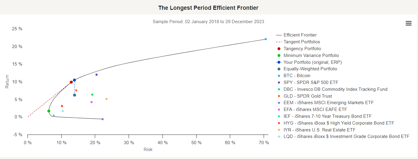
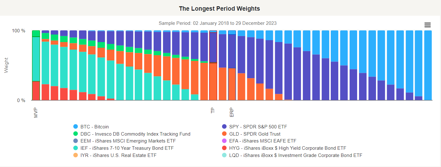
Next, we used the Markowitz Model to analyze portfolio combinations based on expected returns and standard deviations (variance). The Longest Period Efficient Frontier chart displays portfolios with all the different combinations of assets that result in efficient portfolios (i.e., with the lowest risk, given the same return, and portfolios with the highest return, given the same risk). Risk is depicted on the X-axis, and return on the Y-axis.
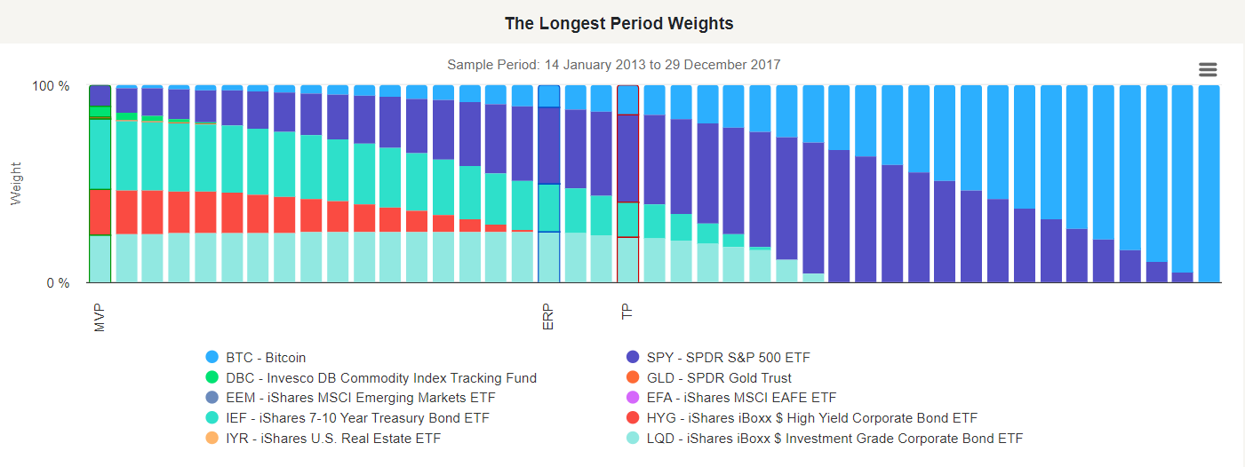
The Efficient Frontier chart also displays the Tangency portfolio – the optimal portfolio that realizes the highest possible Sharpe ratio, Minimum Variance portfolio – the portfolio with the lowest risk and Equal Risk Portfolio (ERP) shows how your portfolio (in this case, our equally weighted portfolio) can be improved in return with the same amount of risk.
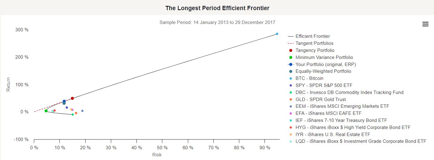
The Tangency portfolio (TP) – the optimal portfolio realizing the highest possible Sharpe ratio – representing the portfolio with the highest risk-adjusted return – tells us to allocate 14,42% to Bitcoin. This tangency portfolio would give us approximately 48.7% return with a 14.97% volatility and respectable Sharpe ratio of 3.25. The portfolio’s extraordinary results are driven mainly by its allocation to Bitcoin. But of course, a minimal number of people had any allocation to Bitcoin at that time, and those times will never return!
Risk Parity
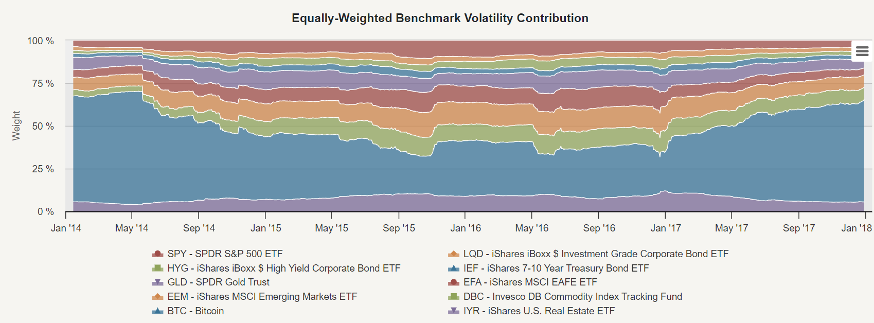
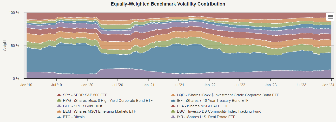
In the next step, we looked into Risk Parity, an investment management strategy focusing on risk allocation. The main aim is to find weights of assets selected in the Portfolio Manager that ensure an equal level of risk for all assets. To allocate the correct risk parity weight to an asset, we must measure its risk (e.g. historical 126-day volatility). This approach helps to reduce the concentration of risk in a few assets and enhances diversification. The initial graph (Equally-Weighted Benchmark Volatility Contribution) shows how much BTC contributed to risk over the years. Over time, BTC remained the main contributor to risk in our equally weighted portfolio.
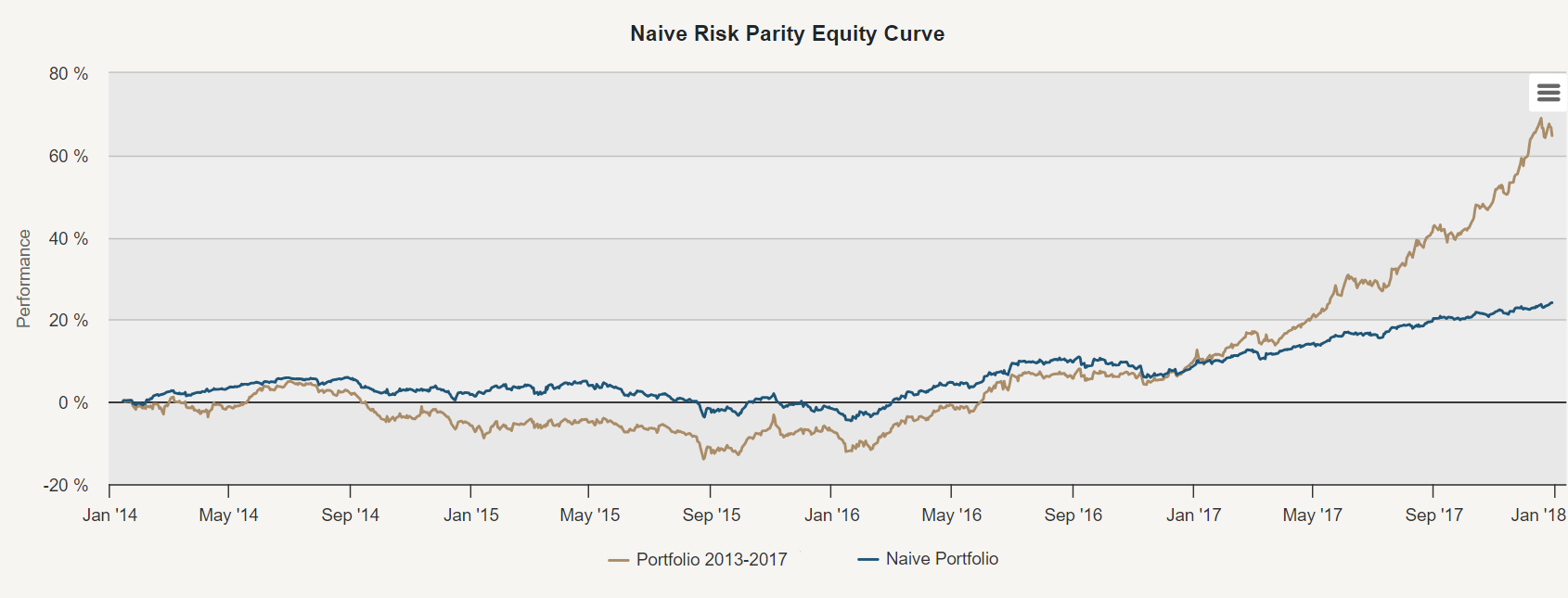
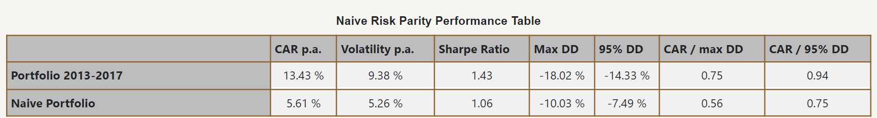
Next, let’s look at the equity curve of the Naive Risk Parity strategy in contrast to our equally weighted portfolio. Naive risk parity or naive risk weighting uses the inverse risk approach instead of equal weights. This approach gives lower weight to riskier assets and greater weight to less risky assets, ensuring that the risk contribution of each asset is the same. As we can see in the Naive Risk Parity Performance Table, this method significantly lowered the strategy’s volatility (from 9.38% to 5.26%). However, this risk reduction came at the expense of lower returns (from 13.43% to 5.61%).
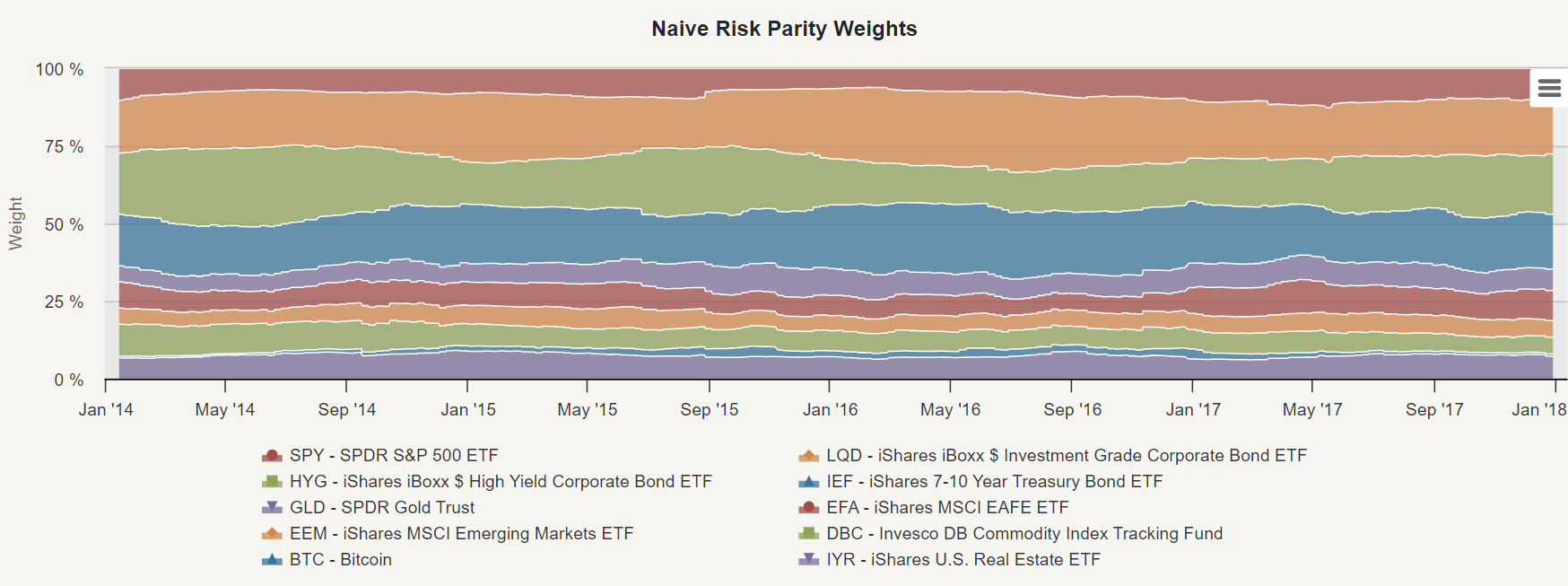
This approach ensures that no single asset, including Bitcoin, dominates the portfolio’s risk exposure. As a result, Bitcoin’s high volatility led to a smaller allocation within the risk parity portfolio to maintain a balanced risk profile across all assets. What’s the Risk Parity’s average allocation to Bitcoin? It’s only approximately 2% due to Bitcoin’s excessively high risk.
2018-2023
In the second part of our analysis, we examined an equally weighted portfolio of the ten assets including Bitcoin from 2018 to 2023. This allocation resulted in an annual return of only 9.05% (compared to 22.86% from the previous period), with a higher volatility of 13.93% (compared to 11.76% of the prior period) and a maximum drawdown of -24.92% (compared to -18.02% from the previous period). Similar to the previous part of our analysis, during the time interval from 2018 to 2023, we conducted a study that examined the Correlation Table, applied the Markowitz Model, and implemented the Naive Risk Parity strategy. So, how much Bitcoin should we allocate to the portfolio based on post-financialization period data?

Underlying Component Analysis
Additionally, in this phase of our analysis, we performed an Underlying Component Analysis to examine the individual performances of various assets within our equally weighted portfolio. This allows us to understand how each asset contributes to portfolio performance throughout the years.
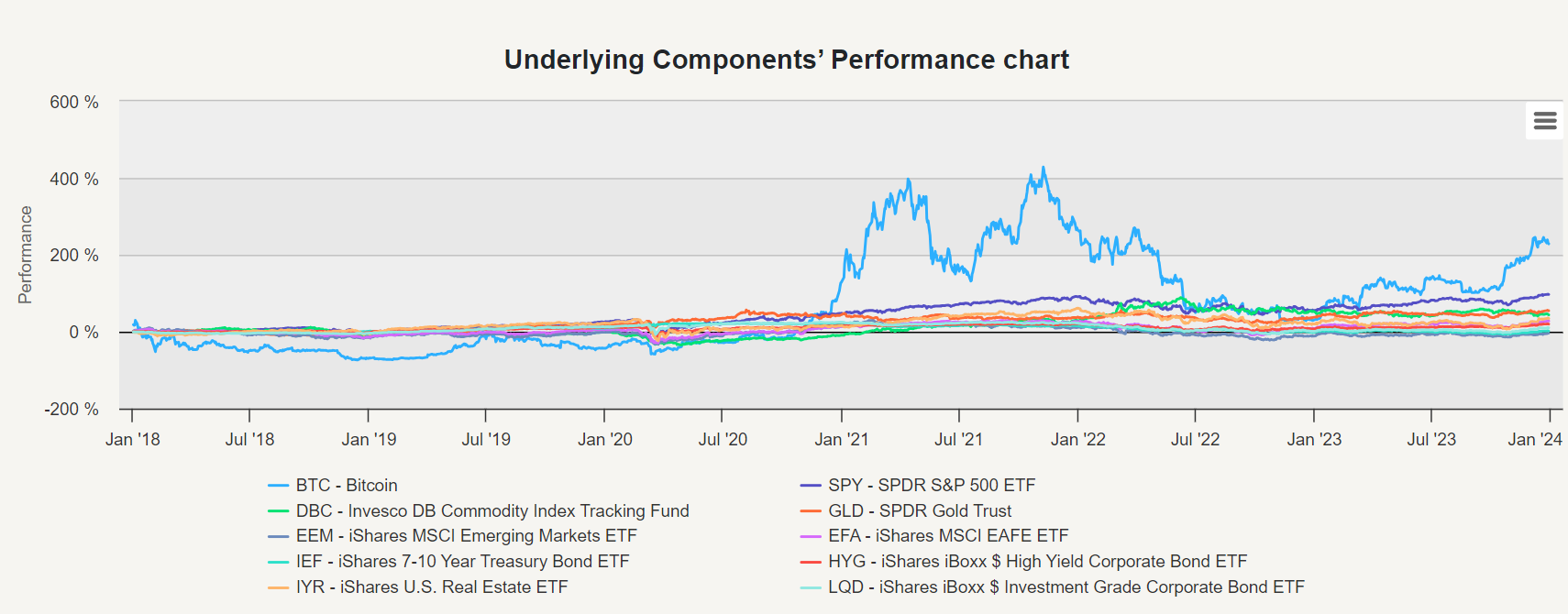
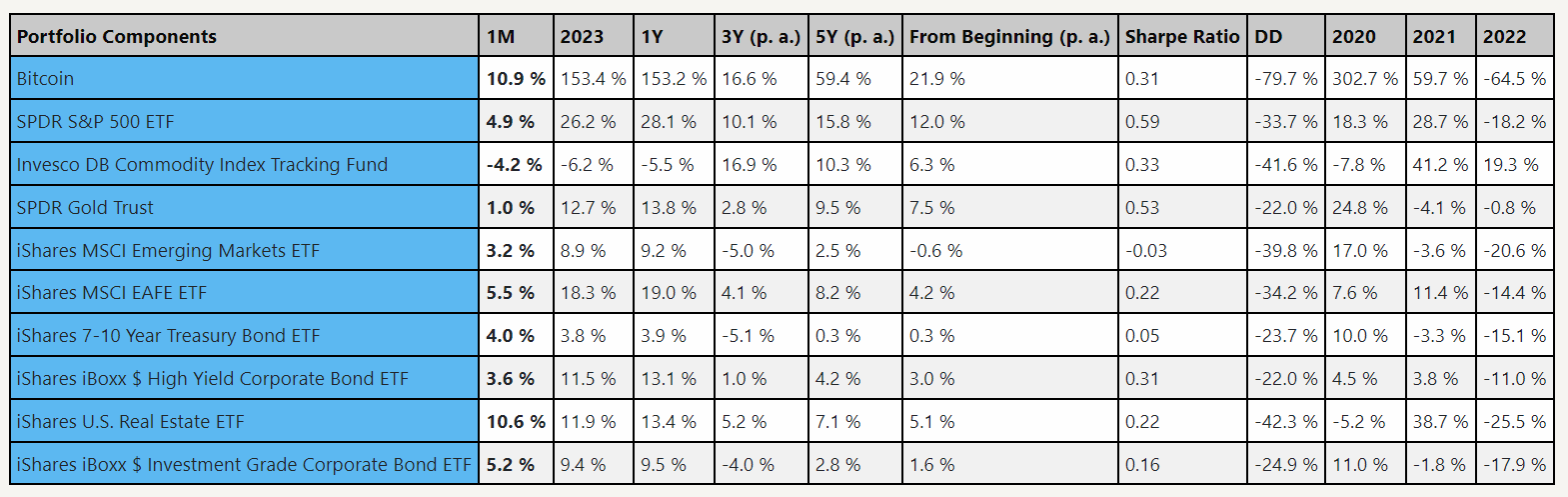
Bitcoin’s post-financialization Sharpe ratio of 0.31 makes it an average asset. It’s outmatched by S&P 500, commodities, and gold and is approximately in the same category as high-yield bonds, MSCI EAFE, or US REITs. Bitcoin had a higher performance but was the most risky asset in the whole portfolio (by a high margin).
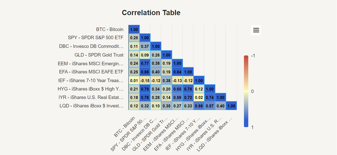
Correlation Table
In the previous part (years 2013-2017), we found that the correlation of Bitcoin with other assets in the Correlation Table ranged from -0.02 to 0.03. As we can see, looking at the different periods, they changed a lot. Bitcoin maintained a consistently low correlation solely with IEF (iShares 7-10 Year Treasury Bond ETF). The highest correlation with SPY (SPDR S&P 500 ETF) and EFA (iShares MSCI EAFE ETF) equals 0.25.
This higher correlation suggests a stronger simultaneous movement or dependency between Bitcoin and these traditional market assets. Such findings are not surprising and underscore the evolving dynamics of Bitcoin’s relationship with mainstream financial instruments. Commodities and emerging markets also had low correlations in the pre-financialization period, and those correlations significantly increased in the post-financialization period. We can expect that the correlation of Bitcoin to the main asset classes will increase even more in the future, and if you intend to allocate to cryptocurrencies, you should include this expectation in your decision process.
Markowitz Model
In applying the Markowitz Model to analyze the portfolio from 2013 to 2017, the Tangency portfolio (TP), representing the optimal portfolio with the highest risk-adjusted return, advised allocating approximately 14.42% to Bitcoin, maximizing the Sharpe ratio. However, the analysis shifted from 2018 to 2023, and the Tangency portfolio suggested allocating only 2.94% to Bitcoin. This adjustment reflects changes in market conditions, risk profiles, and expected returns over the specified period. The Markowitz Model’s analysis acknowledged the decrease in Bitcoin’s performance and simultaneously considered its elevated risk relative to other asset classes. The resultant Tangency portfolio has a 9.82% return and 12.93% volatility, and Bitcoin’s contribution to the performance is minimal (just 0.6%).
Risk Parity
As we can see on the Equally-Weighted Benchmark Volatility Contribution graph for 2018-2023, Bitcoin remained a significant contributor to overall portfolio volatility in equally weighed portfolio. What happens when we run a Naive Risk Parity in this period?
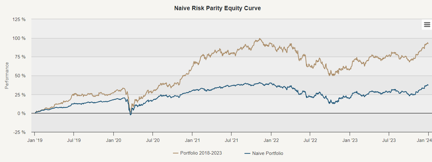
The Naive Risk Parity strategy mitigated some risk, decreasing portfolio volatility from 14.27% to 9.84% compared to the equally weighted portfolio. Once again, this risk reduction was accompanied by a decrease in returns, declining from 14.00% to 6.54%.
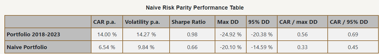
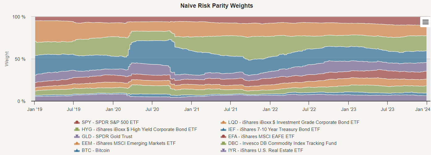
The outcome of the Naive Risk Parity strategy was again a significant decrease in allocation to Bitcoin (once again, to approximately 2%). This adjustment reflects the strategy’s focus on allocating more weight to less risky assets and reducing exposure to riskier ones. By decreasing Bitcoin’s allocation, the strategy aimed to mitigate the impact of Bitcoin’s volatility on the overall portfolio risk.
Conclusion
The comparison between the two periods, 2013-2017 and 2018-2023, reveals a significant shift in the Bitcoin and cryptocurrency investments landscape. During the earlier period, the methods employed, such as the Markowitz Model, may suggest allocating a considerable portion of the portfolio to Bitcoin due to its high return despite its inherent volatility and risk. At the same time, the absence of correlation with other assets underscores the diversification benefits Bitcoin offered in this period. However, as time progressed and the financialization of Bitcoin occurred in December 2017, the dynamics of the cryptocurrency market underwent a fundamental change. Bitcoin and cryptocurrencies became part of the mainstream financial ecosystem, increasing their adoption and recognition as a legitimate asset class while increasing the correlation with mainstream financial instruments.
When optimizing portfolios from 2018 to 2023, Bitcoin is now viewed as average compared to other asset classes and has a relatively high risk. Therefore, while Bitcoin may have shown exceptional growth and returns in its early years, the changing market dynamics and increased institutional involvement have altered its risk-return profile, and our analysis suggests that it’s prudent to cap allocation to Bitcoin (or the whole pool of cryptocurrencies as an asset class) to maximally 2-3% of the portfolio. The higher allocation to this new asset class is probably not justified and bears an unnecessary risk.
The analysis underscores the need for caution and realistic expectations when interpreting historical data and extrapolating long-term conclusions. While past performance may offer valuable insights, it does not guarantee future outcomes, especially in a rapidly evolving and volatile cryptocurrency market. For those interested in learning how to buy Bitcoin, it is essential to thoroughly research and understand the risks involved, ensuring that any investment aligns with their financial goals and risk tolerance.
Authors:
Juliana Javorská, Quant Analyst, Quantpedia
Radovan Vojtko, Head of Research, Quantpedia
Are you looking for more strategies to read about? Sign up for our newsletter or visit our Blog or Screener.
Do you want to learn more about Quantpedia Premium service? Check how Quantpedia works, our mission and Premium pricing offer.
Do you want to learn more about Quantpedia Pro service? Check its description, watch videos, review reporting capabilities and visit our pricing offer.
Do you want algorithmic access to the full Quantpedia database via the API? Subscribe to Quantpedia Pro, ask for an API key, and explore the in/out-of-sample statistics, source academic papers, and code snippets — ideal for quantitative research, systematic trading workflows, and AI model training.
Are you looking for historical data or backtesting platforms? Check our list of Algo Trading Discounts.
Or follow us on:
Facebook Group, Facebook Page, Twitter, Linkedin, Medium or Youtube
Share onLinkedInTwitterFacebookRefer to a friend


