Most of you have probably heard the saying that somebody “averaged” into or out of his investment position. But what does it exactly mean, and what different dollar-cost averaging strategies exist? We plan to unveil our new “Dollar-Cost Averaging” report for Quantpedia Pro clients next week, and this article serves as a short introduction to this term.

What is dollar-cost averaging?

Imagine you won a significant amount of money and you want to invest it in a particular investment. You can either invest it all at once or spread it into multiple smaller investments over time.

If you chose to spread the investments, you picked a strategy called dollar-cost averaging. When an investor applies dollar-cost averaging (DCA), they invest the money in equal portions at periodic intervals, regardless of the market conditions. This way, they eliminate the emotions that come with rising and falling markets. Investors, just like other people, are emotional, so changes in the market prices do affect them. However, mechanically investing at regular intervals takes the emotions out of the equation.

Exactly the opposite way of making regular, piecewise investments – investing all at once – is often called a “lump sum investment”.

Advantages of dollar-cost averaging

In short – diversification. Diversification is the first and the foremost pro of dollar-cost averaging. You diversify your investment across multiple timeframes. Are the markets falling and you’re wondering whether to invest or not? Well, then you don’t have to worry anymore when using DCA. The chances are, that if you divide your investment into enough parts – the markets will not be falling anymore once you finish your partial investments and you may even happen to be buying at lower average price compared to the one-time investment.

Disadvantages of dollar-cost averaging

On the other hand, if the market is rising and you dollar-cost average, you are losing on potential returns you would have gained had you invested your money in a lump sum earlier. Thus, even though investing all your money at once is riskier, it often yields higher returns in the long run.

It was found in a 2012 study by Vanguard that the longer the time frame, the higher the chance that investing all at once beats dollar-cost averaging. Another thing to keep in mind are the brokerage fees, usually linked to every single investment. This may slightly deteriorate performance of DCA, if such fees are high.

Return distribution of dollar-cost averaging

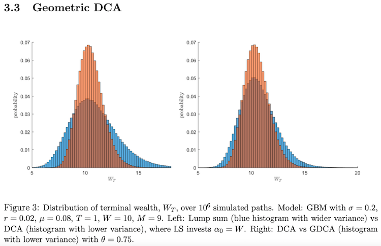
Let’s take a look at the following figure from An Analysis of Dollar Cost Averaging and Market Timing Investment Strategies by Kirkby J., Sovan M., Nguyen, D. This figure shows that Lump Sum has larger tails(blue distribution), meaning it is a riskier investment. On the other hand, Dollar Cost Averaging (orange distribution) has smaller tails, indicating less risk.

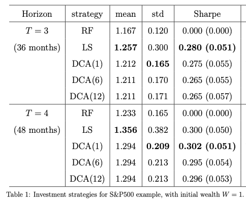
Secondly, we present a table from the same paper. The table compares risk and return of Dollar-Cost Averaging and Lump Sum strategies on a 36-month and 48-month period. Return-wise, Lump Sum wins in both cases. When it comes to Sharpe ratios, we can see that the results are mixed. The Lump Sum strategy has a greater Sharpe ratio in the 36-month period, but DCA has the highest Sharpe ratio in the 48-month period.

Alternative averaging and money management strategies

There are numerous alternative strategies how one may divide or manage their investment. Usually they are much more complex compared to DCA, though.

Firstly, one of the simplest ones is a strategy called value averaging. Value averaging once again smoothens the investment fluctuations, as you buy more shares when prices fall and fewer shares when they rise. However, when the markets trend in one direction, you may become invested too much and too soon (bear trend) or too little and too late (bull trend). 

Secondly, one may apply well-known money management strategies to their investment, after investing it as a lump-sum. Quantpedia has already covered several of these, for example Volatility Targeting, Constant Proportion Portfolio Insurance or Optimal f and Kelly criterion.

Thirdly, one may apply a market timing strategies to their lump sum investment, if they feel insecure about the future development of the underlying.

Our analysis of various dollar-cost averaging strategies

Now, let’s move to our analysis. Firstly, we compare three different DCA strategies to a Lump Sum benchmark. We use SPY (SPDR S&P 500 ETF Trust) data during two time periods to conduct the analysis. The first period is a recent bull market from 20.10.2016 till 20.10.2021. The second period runs from 3.1.2008 till 3.1.2012, this includes the 2008 financial crisis, and serves as a bear market scenario. We set our budget to 10 000$ and make investments on a monthly basis.

3 different strategies

The first DCA strategy invests periodically only during the first half of the period. Therefore, we make 25 investments during the first half and then just hold the entire investment till the end of the period. To better understand the principle, see the following figure, which illustrates how the cash position develops.

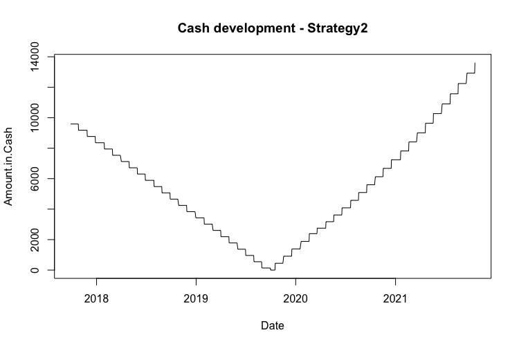
Similarly, the second DCA strategy also invests periodically during the first half of the period. However, it divests during the second half. The divestments are made every month and are calculated as variable monthly payments. So, for example, if the portfolio’s value is 15 000$ the day before we start divesting and there are 15 months till the end of the period, we divide the value into 15 parts worth 1 000$ in the beginning. Then each part appreciates in value individually, and thus each part is divested at a different value. This method is sometimes also called “fixed fractional shares”. Once again, we illustrate the development of cash position visually, so you can better understand the principle of this strategy.

The third and the last DCA strategy invests periodically during the first third of the period, then holds the investment during the second third, and lastly divests on a monthly basis during the last third of the period. The divestments work the same way as in the second strategy. The following figure illustrates the change in cash position to understand the principle of the third strategy better.

Performance of strategies 2016-2021

Let’s now look at the performance of these strategies during the 20.10.2016 – 20.10.2021 period.

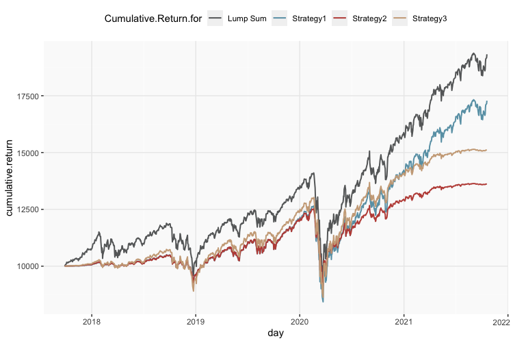
The figure shows the cumulative performance of all three strategies. As we may expect, in the bull market the Lump Sum benchmark performed the best. The table below shows the additional risk and return characteristics of all the strategies and the benchmark.

	Cumulative Return	Volatility	Sharpe ratio	Maximal Drawdown	95% Drawdown	CAR/ Max DD	CAR/ 95% DD
LumpSum.SPY	17.64%	20.48%	0.86	-33.72%	-14.43%	0.52	1.22
DCA.Strategy1.SPY	14.44%	18.52%	0.78	-33.35%	-12.20%	0.43	1.18
DCA.Strategy2.SPY	7.90%	13.87%	0.57	-27.09%	-10.84%	0.29	0.73
DCA.Strategy3.SPY	10.71%	18.42%	0.58	-33.72%	-13.18%	0.32	0.81

As we can see, neither of the DCA strategies outperformed the benchmark Lump Sum strategy. Nonetheless, if we look at the second period we analyzed (3.1.2008 – 3.1.2012), we can see that in the bear market all of the DCA strategies performed better than the Lump Sum benchmark.

Performance of strategies 2008-2012

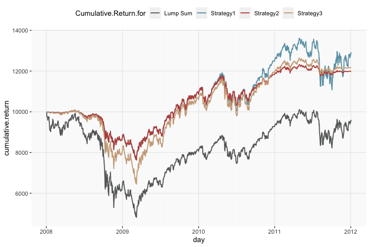
The 2008 crisis is exactly the period when DCA strategies outperformed Lump Sum significantly. The strategies gradually increased the invested amount and hence avoided part of the bear market, averaging down on the prices. In the table below, we can also analyze the risk and return characteristics during this period.

	Cumulative Return	Volatility	Sharpe ratio	Maximal Drawdown	95% Drawdown	CR/ Max DD	CR/ 95% DD
LumpSum.SPY	-1.01%	28.59%	-0.04	-51.85%	-40.71%	-0.02	-0.02
DCA.Strategy1.SPY	6.63%	18.13%	0.37	-24.20%	-16.30%	0.27	0.41
DCA.Strategy2.SPY	4.63%	13.07%	0.35	-24.19%	-15.78%	0.19	0.29
DCA.Strategy3.SPY	5.02%	18.98%	0.26	-36.16%	-23.59%	0.14	0.21

DCA applied to Bitcoin during sideways of 2018-2020

Lastly, we analyzed the BTC (Bitcoin USD) during a period from 2.1.2018 till 2.11.2020. Once again, we started with a budget of 10 000$ and applied the same three DCA strategies. The only difference is that we invest (/divest) on a weekly basis. The following figure shows the cumulative performance of the three strategies and the Lump Sum benchmark.

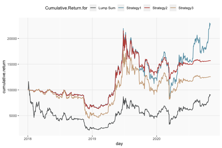
Overall, all three DCA strategies outperformed the benchmark during this sideways period. Now, let’s examine the table of the risk and return characteristics.

	Cumulative Return	Volatility	Sharpe ratio	Maximal Drawdown	95% Drawdown	CR/ Max DD	CR/ 95% DD
LumpSum.BTC	-3.48%	72.91%	-0.05	-81.40%	-78.58%	-0.04	-0.04
DCA.Strategy1.BTC	33.79%	57.12%	0.59	-61.61%	-44.22%	0.55	0.76
DCA.Strategy2.BTC	17.21%	41.27%	0.42	-43.74%	-37.18%	0.39	0.46
DCA.Strategy3.BTC	8.40%	53.33%	0.16	-56.45%	-50.63%	0.15	0.17

Historical Simulations of various DCA strategies

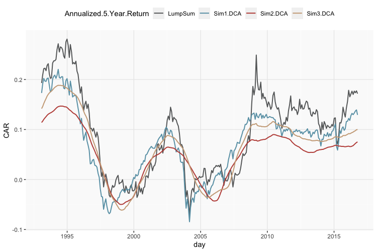
In the second section of our analysis, we simulate rolling 5-year periods from 2.1.1993 till 5.10.2021 (meaning the last period starts 5.10.2016), so that we can see how DCA performs compared to Lump Sum at different points in time. Again, we use SPY (SPDR S&P 500 ETF Trust) data for the simulations. And we analyze the same three DCA strategies as in the first section.

The first figure shows the chart of cumulative performance of SPY during rolling 5-year periods. The dates on the x-axis are the first days of each 5-year period. As we can see, the cumulative return of the Lump Sum benchmark compared to the three DCA strategies varies in time. There are multiple periods where one or more DCA strategies outperform the benchmark. However, we cannot say that the outperformance is consistent. It’s highly dependent on the occurrence of a specific market scenario (usually the falling or sideways one).

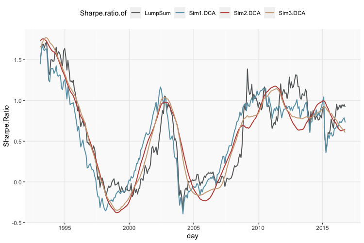
The second figure we present is the chart of rolling Sharpe ratios. Once again, the dates on the x-axis represent first days of each 5-year period. And as we can see, the Sharpe ratios of all three DCA strategies and the Lump Sum benchmark strategy develop similarly over time with brief periods of over and under performance depending on the market scenario.

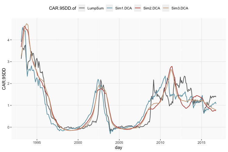
The last figure we present is the chart of rolling ratio of CAR/95%DD. The dates on the x-axis represent first days of each 5-year period. Here, the ratios of all three DCA strategies often outperform the Lump Sum benchmark strategy over several time periods, indicating that this risk-return metric can often be enhanced nicely by using DCA scheme.

Conclusion

As expected, DCA strategies primarily lower the risk thanks to their time diversification properties. This, however, usually comes at the cost of lower returns.

Overall, one cannot say that there is a significant or consistent outperformance of the DCA strategies, nor of the Lump Sum strategy. The performance strongly depends on the market conditions. If an investor expects the markets to fall, it might be wise to apply DCA. Moreover, if one prefers lower risk and lower volatility, DCA might be a good choice as well.

On the other hand, if the only thing an investor cares about is maximizing return, then Lump Sum should be a better choice. At the same time, if one doesn’t have any specific assumptions about future market conditions, in the long run it may be better to invest in a Lump Sum due to statistically higher long-term returns.

Author:
Daniela Hanicova, Quant Analyst, Quantpedia

---

Are you looking for more strategies to read about? Sign up for our newsletter or visit our Blog or Screener.

Do you want to learn more about Quantpedia Premium service? Check how Quantpedia works, our mission and Premium pricing offer.

Do you want to learn more about Quantpedia Pro service? Check its description, watch videos, review reporting capabilities and visit our pricing offer.

Are you looking for historical data or backtesting platforms? Check our list of Algo Trading Discounts.

---

Or follow us on:

Facebook Group, Facebook Page, Twitter, Linkedin, Medium or Youtube

Share onLinkedInTwitterFacebookRefer to a friend