We present a short article as an insight into the methodology of the Quantpedia Pro report – this time for the Markowitz Portfolio Optimization. As usually, Quantpedia Pro allows the optimization of model portfolios built from the passive market factors (commodities, equities, fixed income, etc.), systematic trading strategies and uploaded user’s equity curves. The current report helps with the calculation of the efficient frontier portfolios based on the various constraints and during various predefined historical periods. The backtests of the periodically rebalanced Minimum-Variance, Maximum Sharpe Ratio and Tangency portfolios will be available at the beginning of July.
Additionally, there is a Case Study dedicated to this Quantpedia Pro tool.
Introduction
Markowitz model was introduced in 1952 by Harry Markowitz. It’s also known as the mean-variance model and it is a portfolio optimization model – it aims to create the most return-to-risk efficient portfolio by analyzing various portfolio combinations based on expected returns (mean) and standard deviations (variance) of the assets.
There were several assumptions originally made by Markowitz. The main ones are the following: i) the risk of the portfolio is based on its volatility (and covariance) of returns, ii) analysis is based on a single-period model of investment, and iii) an investor is rational, averse to risk and prefers to increase consumption. Therefore, the utility function is concave and increasing. Additionally, iv) an investor either minimizes their risk for a given return or maximizes their portfolio return for a given level of risk.
When an investor searches for the best portfolio in terms of return-to-risk among the variety of possible portfolios, two steps have to be conducted. The first one is to determine the set of efficient portfolios. The second one is to select the specific, final portfolio from the efficient set, given investor’s target return, target risk or preference toward optimal return-to-risk ratio.
One might ask how to select an optimal portfolio. Basically, from portfolios with the same return, we pick the one with the lowest risk. On the other hand, from portfolios with the same risk level, we choose the one with the highest rate of return.
The efficient portfolios
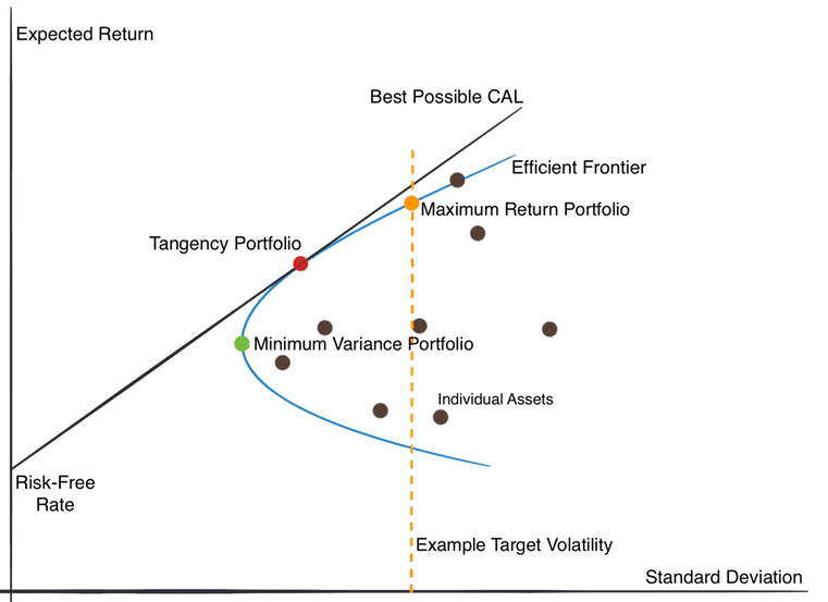
The Efficient Frontier is a hyperbola representing portfolios with all the different combinations of assets that result into efficient portfolios (i.e. with the lowest risk, given the same return and portfolios with the highest return, given the same risk). Risk is depicted on the X-axis and return is depicted on the Y-axis. The area inside the efficient frontier (but not directly on the frontier) represents either individual assets or all of their non-optimal combinations.
Tangency portfolio, the red point in the picture above, is the so-called optimal portfolio that realizes the highest possible Sharpe ratio. As we move from this point either to the right or to the left on the frontier, the Sharpe ratio, or in other words, the excess return-to-risk, will be lower.
The point where the hyperbola changes from convex to concave is where the minimum variance portfolio(green point in the picture) lies.
For a given level of volatility, there also exists a so-called maximum return portfolio (orange point in the picture), which, as the name suggests, maximizes the return given the level of volatility.
Let us now introduce the linear Capital Market Line (CML). The point where the CML meets the Y-axis is where an investor’s risk-free asset, like government securities, lies in terms of the return. This line is tangent to the efficient frontier exactly at the Maximum Sharpe portfolio point. The CML (tangency) line then represents a portfolio of different combinations of a risk-free asset and a tangency portfolio (also called a maximum Sharpe portfolio or sometimes an “optimal portfolio”).
Calculation
When it comes to the math, an efficient frontier can be calculated explicitly, i.e. analytically, only in the simplest case of only one constraint being the sum of asset weights equal to one. Once you start imposing more constraints on asset weights, an optimization procedure needs to be used for calculation of the frontier and the frontier may deviate from the original hyperbola to different curves, given the new constraints. There may be special cases when the solution is explicit, but generally it isn’t.
One of the simplest ways to calculate the efficient frontier under constraints is by using Markowitz’s Critical Line Algorithm (CLA). Unlike some quadratic optimizers, this method works well even if the number of assets N is much greater than the number of observations T. The main idea of CLA is based on a few simple steps. Firstly, you start with the asset with the greatest return, at the upper right side of the Efficient Frontier. Then you follow the Efficient Frontier to the left by looking for the next best asset to be added in or removed one by one.
Numerous curved lines (critical lines), formed by connecting the “corner points”, now form the Efficient Frontier. The portfolios on one critical line, including the corner points, contain same pairs of assets. The only thing that changes are the weights. The set of all critical lines and corner points build up the Efficient Frontier, beginning at the upper right point to the Minimum Variance solution at the far left. Assuming the number of assets, n (n <= N), in the optimal portfolio at a critical line segment is less than the number of observations T (thus n<T), there is a unique solution for CLA.
Markowitz Model in Practice
We decided to investigate the Markowitz model also in practice. We picked four ETFs that serve as building blocks for our portfolios: SPY (US equities), EFA (EAFE equities), GLD (Gold) and IEF (US 7-10y bonds).
Efficient frontier with no constraints
Firstly, we plot a baseline example of the efficient frontier without constraints on assets’ weights and various portfolios associated with the Markowitz’s portfolio theory. Obviously, in all examples there’s always a constraint of the weights summing up to 1. A 1-year calculation period from 8.1.2019 till 8.1.2020 is chosen to demonstrate this example. We use the fPortfolio package in R to calculate the efficient frontier. Additionally, we calculate the weights of the Minimum variance portfolio, Tangency portfolio and Maximum return portfolio with a given level of volatility (set at 6% p.a.), as well as the risk and return of these portfolios. The figure below also shows the 100% SPY, 100% EFA, 100% GLD and 100% IEF portfolios.
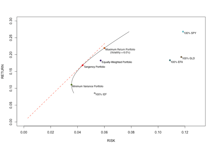
As always, the x-axis shows the annualized values of volatility, and the y-axis shows the annualized values of return. We may observe several interesting phenomena. Firstly, all risky assets are located in the far-right part of the chart, due to their high volatility. Secondly, the displayed part of the efficient frontier, as well as all three displayed portfolios do exhibit much lower volatility than risky assets. This is due to the “no constraints” property of the frontier, i.e. ability to “go short”, i.e. use negative weights for risky assets.
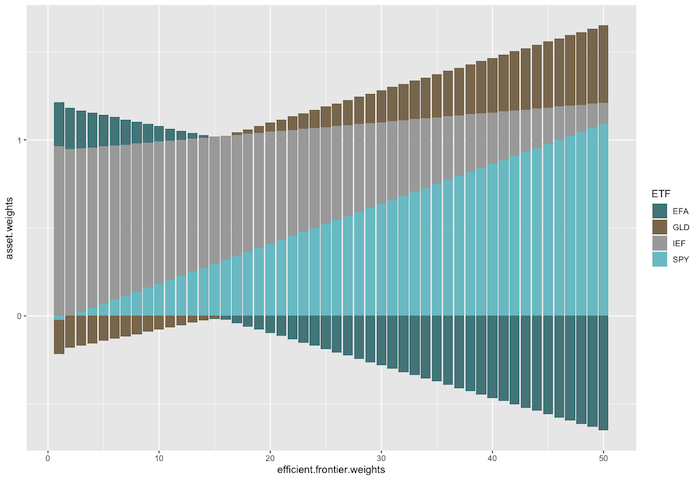
Let’s now take a look at the weights of the ETFs that form the portfolios on the efficient frontier. The following chart shows different asset weights of these portfolios at discrete steps, starting from the southernmost point on the frontier and ending at the northernmost one. We may observe that, e.g. the Minimum variance portfolio is composed primarily of the fixed income ETF, whereas the “northern” part of the frontier consists mostly of risky assets.
Efficient frontier in different times
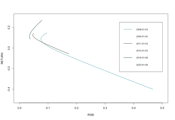
The second plot we analyze shows the evolution of the efficient frontier in time. We picked three time periods: 3.1.2008 – 2.1.2009, 3.1.2011 – 3.1.2012 and 8.1.2019 – 8.1.2020 to demonstrate the changes in time.
As we may see, the efficient frontier varies significantly in time. Apparently, the least volatile frontier with the highest return is the most recent one (2019-2020), while the opposite is true for the oldest frontier (2008-2009). The shape of the curve varies as well.
Efficient frontier with various constraints
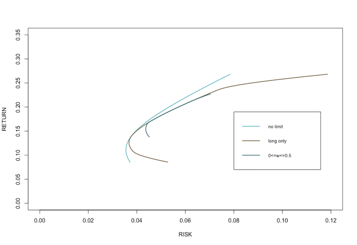
The third example shows how the constraints on the weights of the assets change the shape of the efficient frontier. For this example, we picked the same time period as in the first example (8.1.2019 – 8.1.2020). Three scenarios are examined in the chart below. The only constraint that applies to all three is, that the sum of the weights is equal to one. The first curve is the efficient frontier with no constraints on the weights. The second curve is bind by the long-only scenario, i.e. non-negative weights. In the last scenario (third curve), each asset’s weights are constrained to be non-negative and not greater than 0.5.
The chart below shows the difference in efficient frontiers as a result of different asset weights’ constraints. We can see that the efficient frontier without limit on weights is smoother than the other two (and is the only hyperbola in its true sense). As we add more and more constraints, the frontier naturally moves more “to the right”, i.e. towards higher risk and lower return and changes its shape away from a standard hyperbola.
Trading strategies based on Markowitz
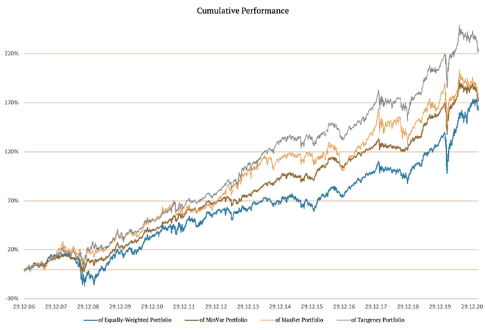
Lastly, we analyze three different trading strategies based on the Markowitz’s model. We test how the periodically calculated Minimum variance portfolio, Tangency portfolio and Maximum return portfolio with a given level of volatility (10% p.a.) perform over time. We compare our results to the equally-weighted portfolio as a benchmark.
We applied the following constraints on the weights: each asset’s weight is non-negative and not greater than 0.5. The rebalance frequency is monthly and the lookback window is 1 year. In other words, each month the weights of the assets of a given portfolio are calculated from the past one-year of data. Finally, the performance of the portfolio is calculated on the daily basis with a 1-day implementation lag to reflect real life conditions.
To sum up, once a month we calculate the Minimum variance, Tangency and Maximum return portfolio and we repeat the process with a moving 1-year data window to arrive at the equity curve of these 3 trading strategies. The following chart shows the cumulative performance of each of the mentioned strategies.
Let’s now take a look at risk and return metrics in a more quantitative manner:
|
|
14Y CAR |
14Y |
Sharpe |
Max DD |
95% DD |
CAR/ |
CAR/ |
|
Equally-Weighted |
7.38% |
11.59% |
0.64 |
-29.58% |
-14.83% |
0.25 |
0.50 |
|
Minimum Variance |
7.64% |
7.14% |
1.07 |
-16.77% |
-5.20% |
0.46 |
1.47 |
|
Tangency Portfolio |
8.96% |
8.63% |
1.04 |
-15.89% |
-6.49% |
0.56 |
1.38 |
|
Maximum Return |
7.78% |
10.26% |
0.76 |
-17.72% |
-9.77% |
0.44 |
0.80 |
As expected, the Minimum variance portfolio has the lowest volatility. The rest of the results are less obvious and may vary in time. Even though the Tangency portfolio has the highest 14-year performance, the Minimum variance portfolio has the highest Sharpe ratio. Overall, all of the portfolios created by the Markowitz’s model performed better than the equally-weighted portfolio in this case – both in terms of return and even more so in terms of risk-adjusted returns. The strategies implicitly combine momentum and low volatility effects, which seem to be to their benefit.
If you’d like to learn even more about the Markowitz Portfolio Optimization, feel free to check out this Case Study.
Author:
Daniela Hanicova, Quant Analyst, Quantpedia
Are you looking for more strategies to read about? Sign up for our newsletter or visit our Blog or Screener.
Do you want to learn more about Quantpedia Premium service? Check how Quantpedia works, our mission and Premium pricing offer.
Do you want to learn more about Quantpedia Pro service? Check its description, watch videos, review reporting capabilities and visit our pricing offer.
Are you looking for historical data or backtesting platforms? Check our list of Algo Trading Discounts.
Or follow us on:
Facebook Group, Facebook Page, Twitter, Linkedin, Medium or Youtube
Share onLinkedInTwitterFacebookRefer to a friend