
Optimal Market Making Models with Stochastic Volatility
Recently, significant developments have occurred in quantitative trading strategies for the execution of the assets in the financial markets by dynamical programming approaches with a very high speed (in microseconds). One of these techniques is called as high-frequency trading (HFT) which has gained excessive attention for its positive impact on the market microstructure. The emergence of HFT has led to the improvements of the numerous algorithmic trading strategies. Consequently, there is a growing demand for quantitative analysis and optimization techniques to develop these strategies.
Aydoğan et al. (2022) works on the derivation of the optimal prices for HFT to execute the limit buy and sell orders where the mid prices of the assets in the market are generated by a stochastic volatility model. Moreover, they add jump components in the dynamics of the prices to measure the effect of number of the arrival orders in the price. More specifically, the goal is to maximize the investor’s expected final wealth at the end of the trading session with constrained inventories. The wealth and inventory processes of the investor during the trading are changing with respect to the arrived and filled orders. The study is the extension of the paper Cartea and Jaimungal (2013) where they study the constant volatility case without drift. Aydoğan et al. (2022) consider the stochastic volatility followed by Heston model consisting jumps either in price or volatility and then they generate the optimal bid and ask prices using stochastic control tool. Since the volatility of an asset is fluctuating, deriving optimal strategies with stochastic volatility in the price dynamics reflects the reality better in the financial markets. To obtain the optimal prices, they solve a highly nonlinear equation which is called as Hamilton-Jacobi-Bellman (HJB) equation proposing an ansatz by the final condition. Then, they apply finite differences and interpolation/extrapolation methods. After obtaining a solution for the stochastic optimal control problem, the findings are performed on an artificial high-frequency data. The results can be applied for HFT even in an emerging market. The models and results presented in this work will serve as extended models for HFT for optimal market making.
Authors: Burcu Aydoğan, Ömür Uğur, and Ümit Aksoy
Title: Optimal Limit Order Book Trading Strategies with Stochastic Volatility in the Underlying Asset
Link: https://link.springer.com/article/10.1007/s10614-022-10272-4
Abstract:
In quantitative finance, there have been numerous new aspects and developments related with the stochastic control and optimization problems which handle the controlled variables of performing the behavior of a dynamical system to achieve certain objectives. In this paper, we address the optimal trading strategies via price impact models using Heston stochastic volatility framework including jump processes either in price or in volatility of the price dynamics with the aim of maximizing expected return of the trader by controlling the inventories. Two types of utility functions are considered: quadratic and exponential. In both cases, the remaining inventories of the market maker are charged with a liquidation cost. In order to achieve the optimal quotes, we control the inventory risk and follow the influence of each parameter in the model to the best bid and ask prices. We show that the risk metrics including profit and loss distribution (PnL), standard deviation and Sharpe ratio play important roles for the trader to make decisions on the strategies. We apply finite differences and linear interpolation as well as extrapolation techniques to obtain a solution of the nonlinear Hamilton-Jacobi-Bellman (HJB) equation. Moreover, we consider different cases on the modeling to carry out the numerical simulations.
Now, we present several interesting figures and tables:


Notable quotations from the academic research paper:
“Figure 2 illustrates the optimal prices for q=-4, q=0 and q=4 where each of them are obtained from one simulation and it shows that how the optimal prices calculated by the spread formulas change by our model. It is observed that the optimal spreads have different asymmetries for different level of the inventories. For example, the strategy is followed as that the trader buys an asset with lower spread and closer price to the midprice while she sells the asset putting higher sell spread and farther price when q=-4. Here, S denotes the midprice of the stock which is obtained by the Heston stochastic volatility model while “bid and ask” denote the optimal bid and ask prices.
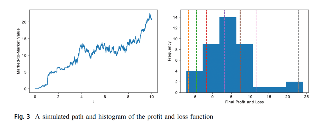
Figure 3 depicts one simulation of the profit and loss function of the market maker at any time t during the trading session in the left panel. The profit and loss performance of the trading is displayed by the cash level histogram in the left panel. It is observed from Fig. 3 that the strategy is profitable even when there are adverse selection effects in the model due to the expectations of the jumps.
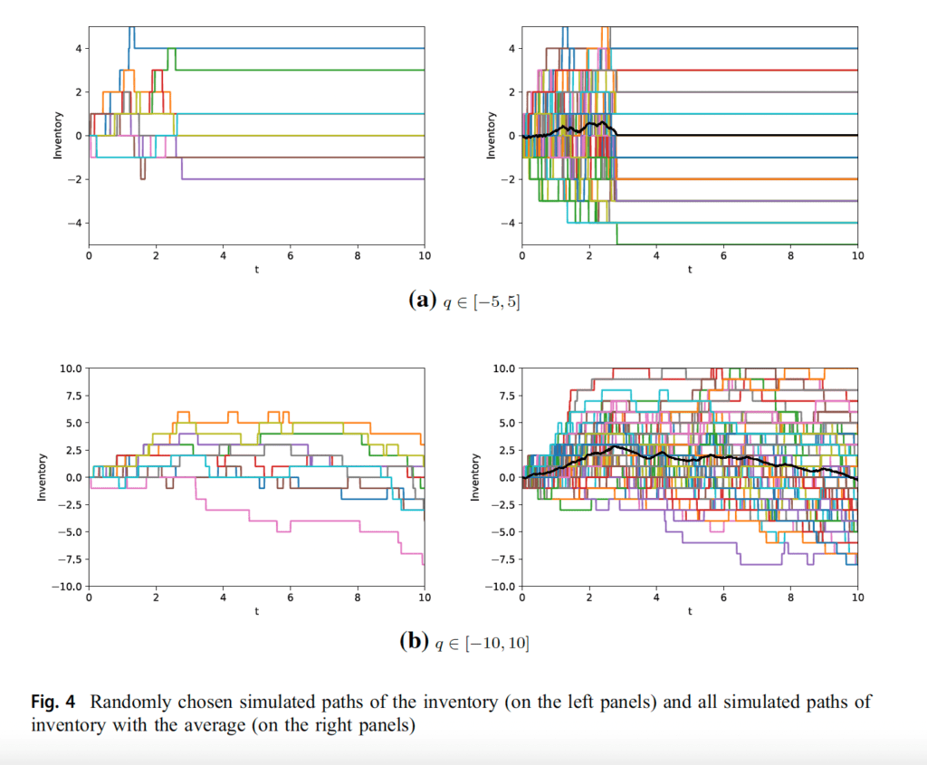
In Fig. 4, some simulated paths of the inventory process and the average of these simulations can be seen for q in [-5, 5] and q in [-10, 10] while the other parameters are fixed. In the left figures, randomly chosen 10 paths of the inventory process are observed. The right figures illustrate all simulated paths with the average of these simulations. It is observed that the inventory processes change for each trade and the summarized pattern tends to revert to zero as the time approaches to the end of the trade. The figure clearly shows that the trade ends at some time between t=2 and t=3 for q in [-5, 5]. We observe this result because the trader’s allowed inventory bound is restricted on a small range, so the inventories may not revert to zero at the end of the trade and she may have to pay the liquidation cost for the remaining inventories. Therefore, we provide the plots for q in [-10, 10] in order to see the time evolution of the process for larger inventory bounds.
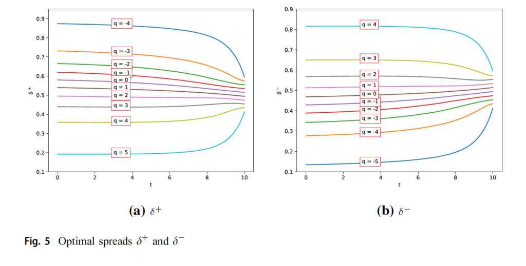
In Fig. 5, we can see the optimal spreads for the trader depending on the each inventory levels with a given liquidation parameter 0.01. This is a small inventory-risk aversion value but is enough to force the inventory process to revert to zero at the end of the trading.
On the negative inventory levels, the values of the optimal ask spreads are larger when t<T since she is unable to sell when the inventory approaches to the minimum admitted level q, so that the trader may want to sell her assets only if she receives a large premium for selling on these levels. As t approaches to the final time, it is observed that the optimal sell spreads decrease since she wants to get rid of her assets rather than paying for the liquidation cost at the end of the trading. On the positive inventory levels, the qualitative behavior of the trader is just the opposite of the idea for the negative inventory levels. In this case, the trader wants to reduce the number of shares in her hand. Because if she still has the assets when the time approaches to the maturity time of the trade, then either she will have to sell them with lower price or pay for the liquidation cost at the end. The probability of selling the assets at maturity time is higher than that for the time far away from the terminal time. Therefore, the trader increases the selling spreads on the positive inventory levels as the time is almost close to the final time. Similar interpretation can be adapted for the optimal buy spread (see Fig. 5b).
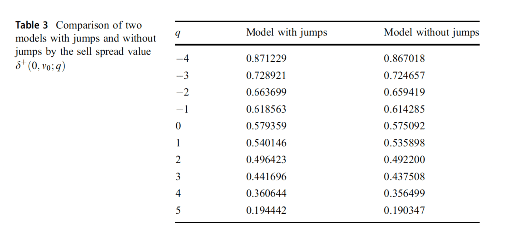
For all simulations, it is observed in Table 2 that, when we compare our strategy with a benchmark strategy that is symmetric around the midprice independently of inventory as done in Avellaneda and Stoikov (2008), profit of the strategy is less than that of the symmetric strategy. On the other hand, the results show that our strategy has a lower standard deviation. It can be also seen that the inventory of the trader reverts to zero more quickly than the symmetric strategy and the standard deviation of the inventory is produced less in the strategy. In Table 3, it is obviously seen that the model with jumps produces larger sell spreads rather than the model without jumps.
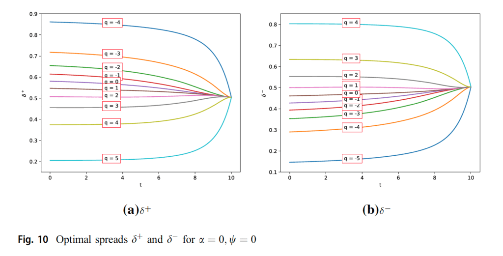
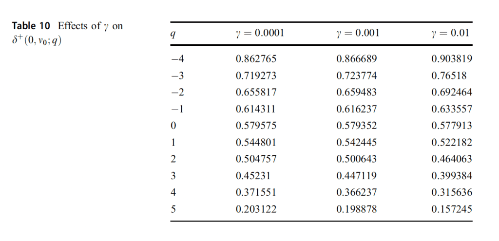
Figure 10 represents the behavior of the trader for zero liquidation cost and zero penalty of the variations on the optimal spreads when the strategy approaches to the terminal time. In this case, since there are no penalizing parameters, it is easy to understand that the spreads converge to a specific value when t approaches to the final time. Table 10 displays the results for the performance of the strategy with a liquidation parameter 0.01.”
Are you looking for more strategies to read about? Sign up for our newsletter or visit our Blog or Screener.
Do you want to learn more about Quantpedia Premium service? Check how Quantpedia works, our mission and Premium pricing offer.
Do you want to learn more about Quantpedia Pro service? Check its description, watch videos, review reporting capabilities and visit our pricing offer.
Are you looking for historical data or backtesting platforms? Check our list of Algo Trading Discounts.
Would you like free access to our services? Then, open an account with Lightspeed and enjoy one year of Quantpedia Premium at no cost.
Or follow us on:
Facebook Group, Facebook Page, Twitter, Linkedin, Medium or Youtube
Share onLinkedInTwitterFacebookRefer to a friend


