The Quant Cycle – The Time Variation in Factor Returns
Although the factors in asset pricing models offer a premium in the long run, they are undergoing bull and bear market cycles in the short term. One would expect that it is due to their connection to the business cycles as the factor premium represents a reward for bearing the macroeconomic risks. A novel study by Blitz (2021) finds that traditional business cycle indicators can’t explain much of the time variation of factor returns as the factors are a behavioral phenomenon driven by investor sentiment. To capture the large factor cyclical variation, the author proposes a quant cycle that is defined by the peaks and troughs in the factor returns corresponding to the bull and bear markets.
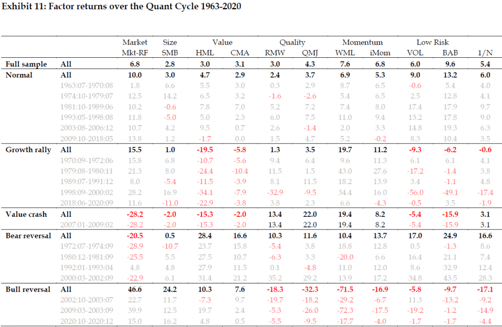
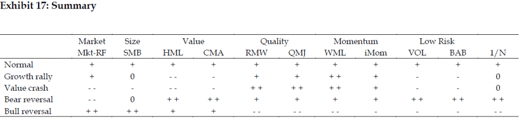
For example, a quant cycle starts with a normal stage that prevails about two-thirds of the time and gets interrupted by a major drawdown of value factor with a periodicity once per ten years. These drawdowns are caused either due to the rally of growth stocks (in a bullish environment) or the crash of value stocks (in a bearish environment). The growth rally is usually followed by a bear reversal, where the growth stocks that rallied during the previous stage crash, resulting in a strong rebound of the value factor. On the other hand, the bull reversal comes after the value crash and is typical for the rebound of the past biggest losers resulting in large negative returns for the momentum factor. Due to the drastic losses for trend-following strategies, bull reversals represent a tough challenge for multifactor portfolios. Therefore, by understanding the quant cycle an investor can form a multi-year outlook and choose the proper factor allocation accordingly.
Author: David Blitz
Title: The Quant Cycle
Link: https://ssrn.com/abstract=3930006
Abstract:
Traditional business cycle indicators do not capture much of the large cyclical variation in factor returns. Major turning points of factors seem to be caused by abrupt changes in investor sentiment instead. We infer a Quant Cycle directly from factor returns, which consists of a normal stage that is interrupted by occasional drawdowns of the value factor and subsequent reversals. Value factor drawdowns can occur in bullish environments due to growth rallies and in bearish environments due to crashes of value stocks. For the reversals we also distinguish between bullish and bearish subvariants. Empirically we show that our simple 3-stage model captures a considerable amount of time variation in factor returns. We conclude that investors should focus on better understanding the quant cycle as implied by factors themselves, rather than adhering to traditional frameworks which, at best, have a weak relation with actual factor returns.
As always we present several interesting figures:
Notable quotations from the academic research paper:
“The factors in asset pricing models exhibit cyclical behavior, offering a premium in the long run, but going through bull and bear phases in the short run. For instance, the HML value factor of Fama and French (1993) has a long-term premium of about 3%, but had a -20% annual return over the 1998-1999 period, followed by a +15% annual return over the 2000-2006 period. What explains these cyclical dynamics of factors?
We argue that factors essentially follow their own cycle, which can be inferred from their realized returns. We determine the quant cycle by qualitatively identifying peaks and troughs that correspond to bull and bear markets in factor returns. Our approach is part art and part science, similar to the fact that there is no universally accepted definition of the bull and bear markets of the equity market. For instance, how deep and how long does a drawdown need to be to classify as a true bear market as opposed to a temporary correction during a bull market?
For defining the Quant Cycle we focus more on volatile factors, such as value and momentum, than on factors such as quality which exhibit much less extreme return swings. Looking at the value factor, we observe that it experiences a major drawdown about once every ten years. The cause for these drawdowns is either a rally of growth stocks (in a bullish environment) or a crash of value stocks (in a bearish environment). These periods also tend to be tough for the low-risk factor. However, as also observed by Blitz (2021), large losses on the value factor are oftentimes mirrored by similar-sized gains on the momentum factor.
Immediately following a growth rally or value crash we typically observe a strong reversal. Here it is even more important to distinguish between bullish and bearish variants, because their impact on factor returns is very different. The first variant, which we will call a bear reversal, is characterized by a crash of the growth stocks that rallied during the previous stage, resulting in a strong rebound of the value factor. An example of this is the burst of the tech bubble in 2000-2002, during which the Nasdaq lost over three-quarters of its value.
The second variant, which we call a bull reversal, is characterized by a rebound of stocks that experienced the biggest losses, resulting in large negative returns for the momentum factor. An example of this is the relief rally of 2009, when cheap financials that were beaten down during the Global Financial Crisis made a strong recovery. A bull reversal can also follow after a bear reversal, if growth stocks that have been massively sold off bounce back again, as in 2002-2003.
Bear reversals tend to be great for multi-factor investors, with large positive returns on all factors, but bull reversals are much more challenging, with large negative returns for most factors except value. After the reversal stage factors tend to revert back to normal mode, which is the stage that actually prevails about two-thirds of the time.
We conclude that in order to understand the cyclical dynamics of factors, investors should recognize that factors follow their own sentiment-driven cycle. Traditional business cycle and sentiment indicators may pick up some of these dynamics, but their practical usefulness is limited. By inferring the quant cycle directly from factor returns we are able to capture much more time variation. The practical implication for investors is that they should focus their efforts on better understanding the quant cycle as implied by factors themselves, rather than adhering to traditional frameworks which, at best, have a weak relation with actual factor returns. An example of a possible application of the model is that it might help investors formulate a multi-year outlook.”
Are you looking for more strategies to read about? Sign up for our newsletter or visit our Blog or Screener.
Do you want to learn more about Quantpedia Premium service? Check how Quantpedia works, our mission and Premium pricing offer.
Do you want to learn more about Quantpedia Pro service? Check its description, watch videos, review reporting capabilities and visit our pricing offer.
Do you want algorithmic access to the full Quantpedia database via the API? Subscribe to Quantpedia Pro, ask for an API key, and explore the in/out-of-sample statistics, source academic papers, and code snippets — ideal for quantitative research, systematic trading workflows, and AI model training.
Are you looking for historical data or backtesting platforms? Check our list of Algo Trading Discounts.
Or follow us on:
Facebook Group, Facebook Page, Telegram, Twitter, Linkedin, Medium or Youtube
Share onLinkedInTwitterFacebookRefer to a friend


