Building and Testing Trend-Following Strategies on One-Minute SPY Data
Intraday trading strategies have gained increasing attention as advances in computing power and market data availability have made intraday strategy analysis more accessible. While many trading strategies are traditionally developed and evaluated using daily price data, shorter timeframes can provide additional opportunities to identify and exploit market trends within a single trading session. In this article, we investigate the performance of trend-following strategies based on selected technical indicators computed from one-minute price data for SPY ETF. The historical dataset, provided by Algoseek, serves as the basis for designing, backtesting, and comparing several intraday trading approaches.
The data
The analysis is based on Algoseek US Equities Trade and Quote Extended Minute Bar data covering the period from April 1, 2021, to April 15, 2026. The dataset contains intraday observations for each trading minute, allowing the development and evaluation of intraday trend-following strategies. Algoseek US Equities Trade and Quote Extended Minute Bar provides minute-level analytics derived from consolidated trade and quote (TAQ) data, with roughly 90 metrics per bar including OHLCV, trade classification at bid, mid, and ask, spread measures, time-weighted quotes, and estimated retail TRF order flow.
One-minute data provide substantially richer market information than is typically available from conventional daily datasets. Besides price and aggregate trading volume, they contain detailed measures describing the composition of trading activity, including retail order flow, off-exchange transactions, and other market microstructure variables. Such information makes it possible to study not only how much an asset traded during the day, but also who was responsible for that trading activity and when it occurred.
This richer view of market structure opens the possibility of identifying relationships that would remain hidden after daily aggregation. Rather than treating each trading day as a single observation, minute-level data allow us to examine how different groups of market participants contribute to price formation throughout the session and whether their activity contains predictive information for subsequent market returns.
Although the dataset includes a wide range of market variables, this article focuses on four key characteristics:
- LastTradePrice – the reference price used for indicator calculation and trade execution.
- RetailTRFBuySize – the estimated retail buy order flow (in shares) reported off-exchange through Trade Reporting Facilities (TRFs).
- RetailTRFSellSize –the estimated retail sell order flow (in shares) reported through TRFs.
- TotalVolume – the total traded volume during the corresponding one-minute interval.
Rather than using the raw retail activity measures directly, we construct two normalized indicators that relate retail trading activity to the total market volume:
RetailRelative = (RetailTRFBuySize + RetailTRFSellSize) / TotalVolume
This indicator measures the proportion of total trading volume attributed to retail participants, regardless of trade direction.
RetailBuyOnly = RetailTRFBuySize / TotalVolume
This indicator captures the relative buying activity of retail traders and can be interpreted as a measure of retail buying pressure.
The windows
An important design decision when developing an intraday trading strategy is determining when a trading signal is generated and how long the resulting position is held. The availability of one-minute data enables us to move beyond the traditional approach of constructing signals from the entire trading day. While daily aggregation is common in quantitative trading, it inevitably discards the temporal structure of intraday market activity. By defining alternative signal windows, we can investigate whether specific parts of the trading session contain more informative signals than others. For example, retail order flow observed shortly after the market opens may reflect investors’ immediate reactions to overnight news and therefore provide an indication of the prevailing sentiment for the trading day.
Rather than continuously opening and closing positions throughout the trading session, we separate the strategy into two independent components: the signal window and the trade window.
The signal window defines the historical intraday period used to evaluate market conditions and generate a trading signal. Three alternatives are considered: 9:30 AM – 3:59 PM (full trading day without last minute, in graphs as D), 3:00 PM – 3:59 PM, (last trading hour without last minute, in graphs as E) and 3:30 PM – 3:59 PM (last trading half-hour without last minute, in graphs as F).
Once the signal has been generated, a long position is opened if the selected trend-following rule indicates a positive trend. The exact construction of the trend-following signal is described in the following section.
The duration for which the position remains open is determined by the trade window. In this study, we focus on two holding periods: 3:59 PM – 9:31 AM (overnight, in graphs as Y3) and 3:59 PM – 3:59 PM on the next trading day (full trading day, in graphs as Y4).
These two holding periods were selected because they represent practical alternatives for systematic traders who seek to exploit daily market movements without engaging in high-frequency trading. Instead of executing a large number of intraday transactions, the strategy generates at most one trading decision per day, based on information accumulated during the selected signal window.
The strategies pool
The proposed strategies are based on the hypothesis that changes in retail trading activity may contain information about future price movements. Instead of deriving trading signals directly from price, we use normalized retail participation indicators calculated over a predefined intraday signal window.
For each trading day, the selected signal is aggregated over the chosen signal window (full day, last hour or last 30 minutes). The resulting daily value is then compared with its historical moving average (in basic setup we use 20 trading days).
A long trading signal is generated whenever the daily indicator exceeds its moving average, suggesting that retail buying activity is stronger than its recent historical average. Otherwise, no position is opened.
Whenever a long signal is generated, the position is entered at the market close (3:59 PM) and held according to the selected trade window. These options (signal & trading window and length of MA window) result in a family of trend-following strategies that differ only in the amount of information used to generate the signal and the duration of the resulting trade.
The first look
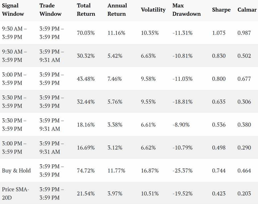
To evaluate the performance of the proposed trend-following approach for relative retail metric, we first analyze a fixed moving average window of 20 trading days. This setting allows us to compare different combinations of signal and trade windows while keeping the trend detection horizon constant.
The strategies are evaluated on the full SPY dataset presented above and compared against two benchmark approaches. The first benchmark is a traditional price-based moving average strategy, where the trading signal is derived directly from the SPY price relative to its 20-day moving average. The second benchmark is a simple buy-and-hold strategy, representing passive exposure to the SPY ETF over the same period.
This comparison allows us to assess whether retail activity-based trend signals provide additional value compared with conventional price-based trend following and passive market exposure.
The results presented in the table and figure below summarize the risk and return characteristics of each approach, including total return, annualized return, volatility, maximum drawdown, Sharpe ratio, and Calmar ratio.
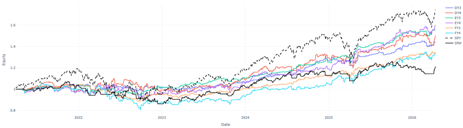
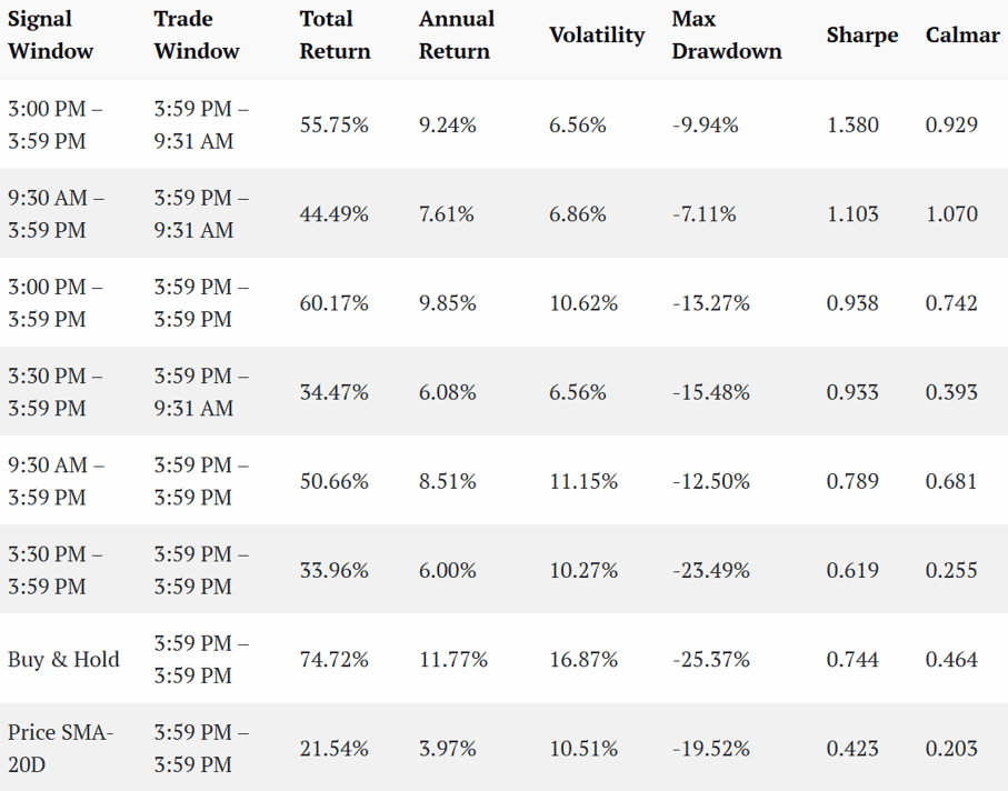
A simple visual inspection of the resulting equity curves shows that the buy-and-hold strategy delivers the highest absolute return over the tested period. If maximizing total return was the only objective, the analysis could arguably end here, with a passive investment in SPY being the most straightforward solution.
However, return alone does not fully describe the quality of a trading strategy. When considering risk-adjusted performance measures such as the Sharpe ratio and Calmar ratio, several of the proposed strategies demonstrate more favorable characteristics compared with both benchmarks. In particular, many retail activity-based trend-following strategies achieve higher risk-adjusted returns while maintaining lower volatility and smaller drawdowns than a simple buy-and-hold approach.
The strongest performance according to the Sharpe ratio is achieved by the strategy using the last-hour signal window (3:00 PM – 3:59 PM) combined with an overnight holding period (3:59 PM – 09:31 AM).
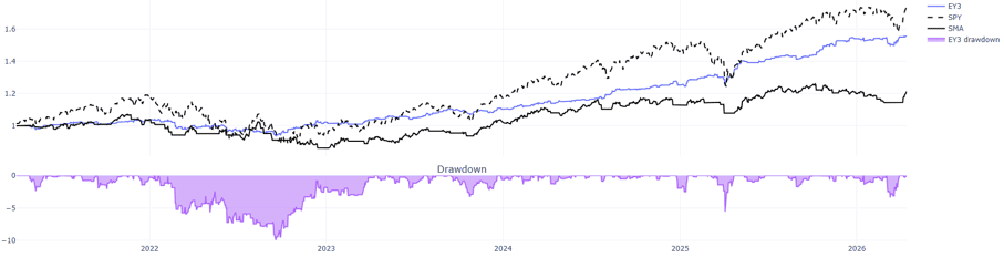
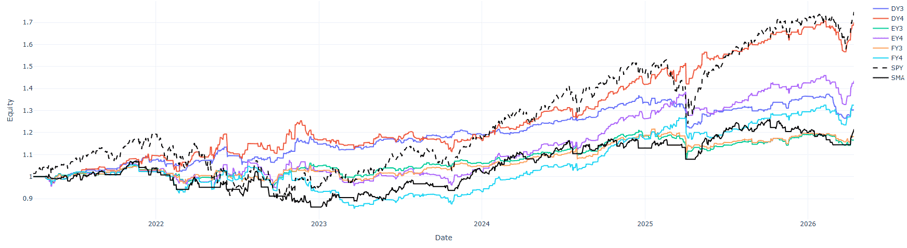
When analyzing the second retail activity indicator, Retail Buy Only, we observe a similar pattern in the results. The majority of tested strategies again achieve improved risk-adjusted performance compared with the benchmark approaches, particularly when evaluated using the Sharpe ratio and Calmar ratio.
The best-performing configuration in this group is the strategy using the full-day signal window (9:30 AM – 3:59 PM) combined with a full trading-day holding period (3:59 PM – 3:59 PM). Unlike the previous set of strategies, this approach achieves a total return that is comparable to the passive buy-and-hold SPY benchmark, while maintaining more favorable risk characteristics.

Focus on robustness
So far, all strategies have been evaluated using a fixed 20-day moving average window. While this provides a consistent basis for comparing different signal and trade windows, a single parameter choice is not sufficient to determine whether the observed performance is robust or merely a result of a specific parameter selection.
To address this issue, we perform an additional robustness analysis by varying the moving average window length and examining how the strategy characteristics change. For each retail activity indicator, we select the three strategies with the highest Sharpe ratio under the 20-day moving average setting and test their performance across alternative moving average horizons.
The objective of this analysis is to evaluate whether the previously observed results remain stable when the trend detection parameter is modified. A robust strategy should maintain relatively consistent risk-adjusted performance across a reasonable range of moving average windows rather than relying on a single optimal parameter value.
For each selected strategy, we provide a graphical visualization showing how the moving average window affects key performance metrics. In addition, for the strategy achieving the highest Sharpe ratio under the 20-day moving average configuration, we present a detailed table summarizing the robustness test results.
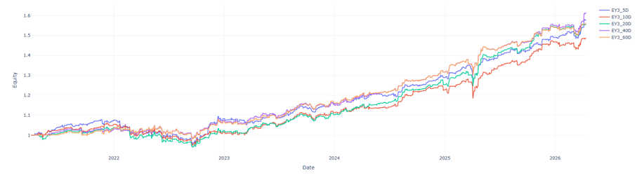
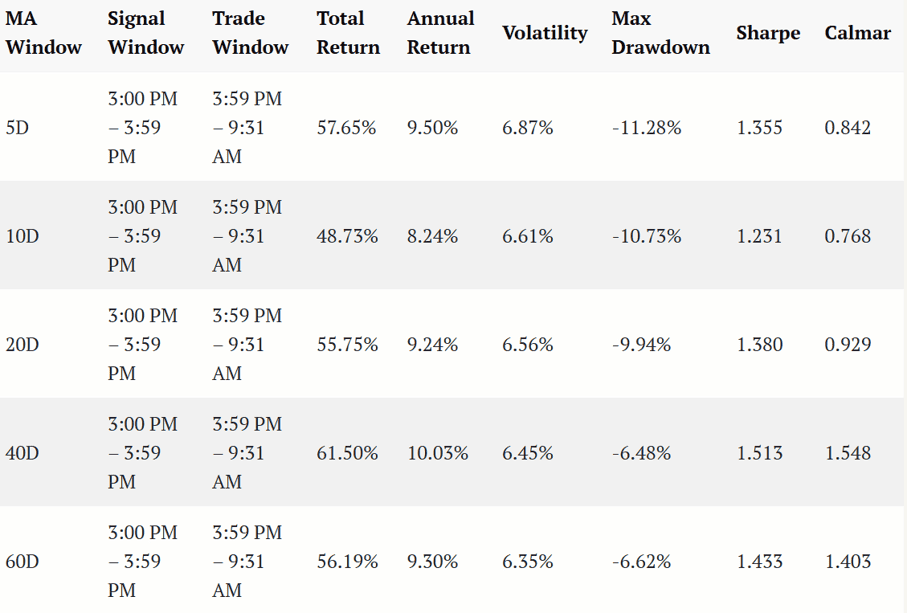
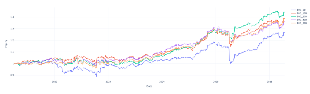
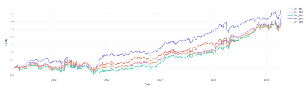
A comparison of the equity curves across different moving average windows reveals a consistent pattern. Although the absolute performance varies with the choice of the moving average horizon, the overall shape of the equity curves remains similar in most cases. The strategies therefore appear to react to the same underlying market dynamics, with the moving average window primarily influencing the magnitude of returns rather than fundamentally changing the trading behavior.
This observation provides additional evidence that the results obtained for the 20-day moving average are unlikely to be the consequence of a single fortunate parameter choice. Instead, the 20-day configuration appears to represent one realization of a broader family of strategies that exhibit similar behavior across a reasonable range of moving average windows. Such consistency increases confidence that the observed performance reflects a more robust relationship rather than an isolated backtesting anomaly.
A similar pattern is observed for the Retail Buy Only indicator. Across all strategy configurations that were previously identified as the strongest under the 20-day moving average setting, the equity curves remain broadly consistent when the moving average window is varied. As in the case of the Relative Retail indicator, the primary differences are reflected in the scale of performance rather than in the overall trajectory of the strategies.
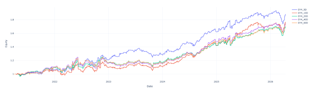
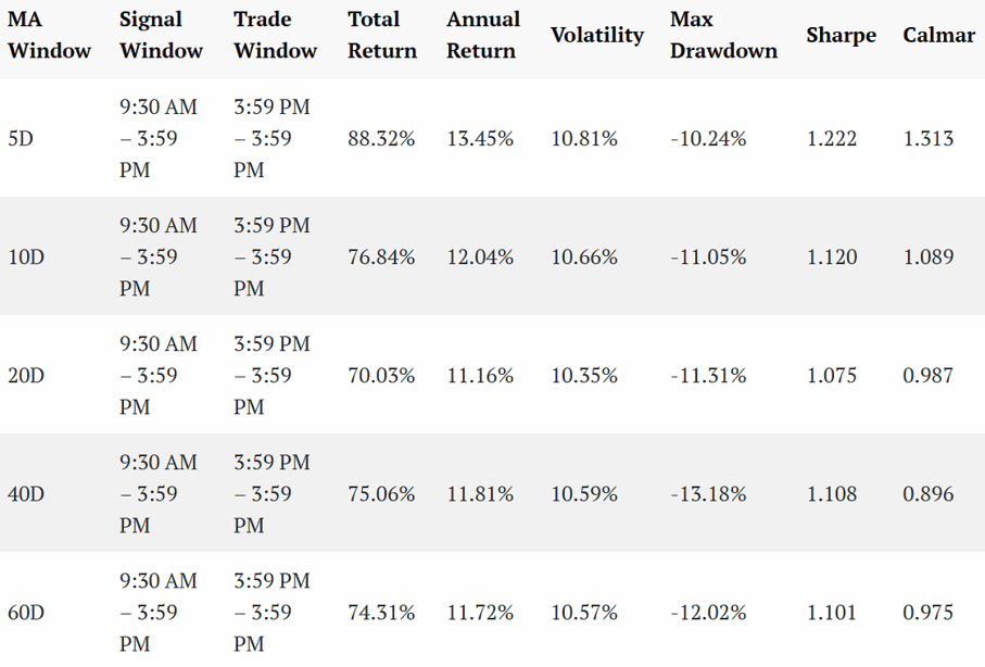
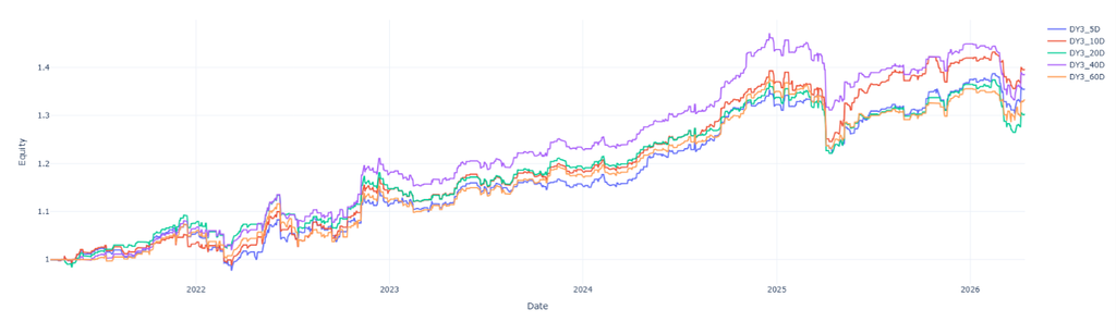
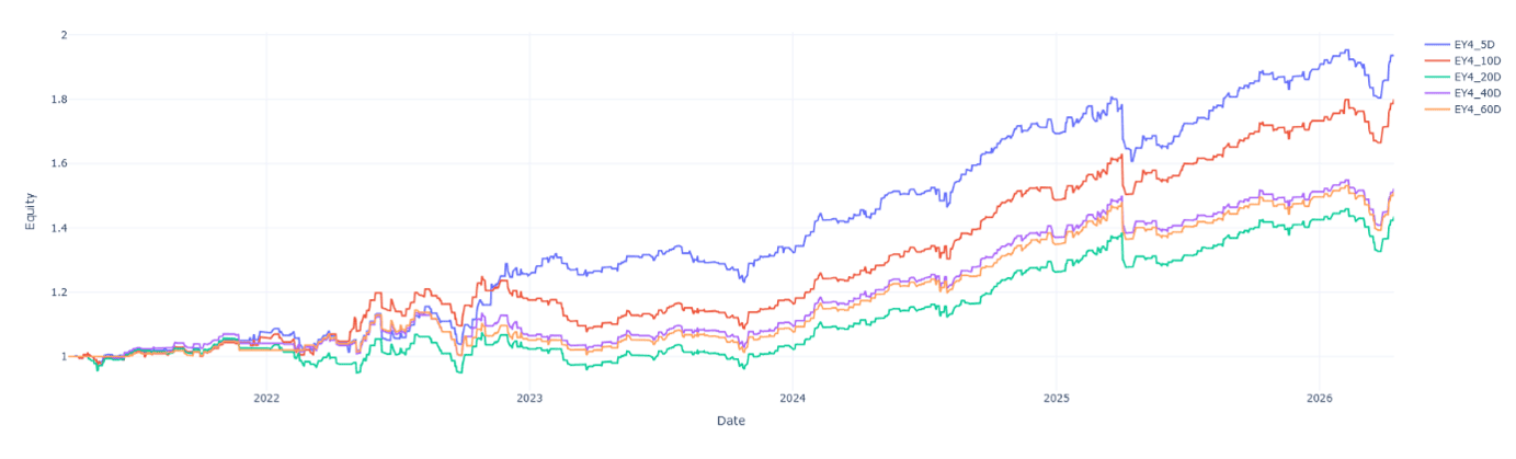
Taken together, these results suggest that the proposed trading rules are not overly sensitive to the specific choice of the moving average horizon. Instead, they exhibit stable behavior across a range of parameter values.
Conclusion
This article investigated whether one-minute SPY market data can be used to construct suitable and robust trading strategies based on end-of-day position entry. The main objective was to examine whether intraday information about market activity can provide additional value when developing systematic trend-following approaches.
We analyzed two retail activity-based indicators derived from minute-level data: the relative share of retail trading activity in total volume and the relative share of retail buying activity in total volume. Based on these indicators, we developed simple trend-following strategies where trading decisions were generated by comparing the current indicator level with its historical moving average.
The results show that the proposed strategies generally provide substantially better risk-adjusted performance. Several tested configurations achieved higher Sharpe and Calmar ratios while maintaining lower volatility and smaller drawdowns compared with passive market exposure.
We also examined the robustness of selected strategies with respect to the moving average window used for signal generation. In most cases, the strategies remain structurally consistent across different parameter choices.
Overall, the results indicate that minute-level retail activity data may contain really useful information for systematic SPY trading strategies. Additionally, our recommendation is, that instead of searching for a single optimal configuration, a more promising direction may be the construction of a composite strategy combining multiple dimensions of the trading process, including the choice of signal window, holding period, and moving average horizon. Such an approach could potentially improve stability and reduce dependence on any individual parameter selection.
Authors:
Jakub Demko, Junior Quant Analyst, Quantpedia
David Belobrad, Junior Quant Analyst, Quantpedia
Are you looking for more strategies to read about? Sign up for our newsletter or visit our Blog or Screener.
Do you want to learn more about Quantpedia Premium service? Check how Quantpedia works, our mission and Premium pricing offer.
Do you want to learn more about Quantpedia Pro service? Check its description, watch videos, review reporting capabilities and visit our pricing offer.
Do you want algorithmic access to the full Quantpedia database via the API? Subscribe to Quantpedia Pro, ask for an API key, and explore the in/out-of-sample statistics, source academic papers, and code snippets — ideal for quantitative research, systematic trading workflows, and AI model training.
Are you looking for historical data or backtesting platforms? Check our list of Algo Trading Discounts.
Or follow us on:
Facebook Group, Facebook Page, Telegram, Twitter, Linkedin, Medium or Youtube