We are really excited that we can announce, that Quantopian started to publish series of articles where they will really deeply analyze some of Quantpedia's suggested strategies.
We think, that Soeng Lee from Quantopian did a really good job with a first article, so we just wanted to point that article to you as something interesting to read for people with an interest in "quant trading". Click on a "View Notebook" button to read a complete analysis:
https://www.quantopian.com/posts/quantpedia-trading-strategy-series-are-earnings-predictable
First article analyses strategy #271 – Earnings Announcements Combined with Stock Repurchases. Quantopian's analysis confirms initial findings of Amini & Singal academic paper:
Earnings are a highly studied event with much of the alpha in traditional earnings strategies squeezed out. However, the research here suggests that there is some level of predictability surrounding earnings and corporate actions (Buyback announcements). In order to validate the authors' research, Soeng Lee from Quantopian attempts an OOS implementation of the methods used in the Amini&Singal whitepaper. He examines share buybacks and earnings announcements from 2011 till 2016 finding similar results to the authors with positive returns of 1.115% in a (-10, +15) day window surrounding earnings. The results hold true for different time windows (0, +15) and sample selection criteria.
Soeng finds the highest positive returns for earnings that are (5, 15) days after a buyback announcement (abnormal returns of 2.67%). Also, the main study by Amini&Singal was focused on buybacks greater than 5%. However, the robustness test that included all buybacks appears to outperform the main study. The test looking at buybacks 1 ~ 30 days before an earnings announcement also performed better than the 16 ~ 31 days criteria (as suggested in Amini&Singal) with a greater sample size.
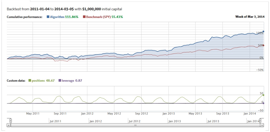
The final Quantopian OOS equity curve looks really promising:
This Quantopian's analysis is the first of the longer series of articles. We are already looking forward to the next one …
