An Analysis of Rebalancing Performance Dispersion
Introduction
The theme of rebalancing in longer-term investing is neglected but important as it influences the overall portfolio’s performance and risk. Unfortunately, many investors are inconsistent in choosing dates for their rebalances of portfolios, resulting in hardly predictable results (whether positively or negatively affecting it), and not contributing to handling risk management properly. The following article presents our analysis of the impact of rebalancing on portfolio returns. It also serves as an introduction to the methodology for an upcoming Quantpedia Pro report that our users would be able to use to quickly assess the impact of the rebalancing period on any selected combination of trading strategies, custom equity curves, and ETFs.
Literature Review
We build our contribution to research and are inspired by our previous reports How Often Should We Rebalance Equity Factor Portfolios? (May 2022) and Better Rebalancing Strategy for Static Asset Allocation Strategies (March 2019). The topic, of course, is very wide, and many approaches can be applied, varying on many dependent variables.
If we look from the view of factor investing and allocation, Flint and Vermaak in their Factor Information Decay: A Global Study (December 2021) propose that the information-optimal rebalance period is 3 − 4 months for Value, 3 months for Momentum, 4 − 5 months for Quality, 1 month for Investment, and 5 − 6 months for Low Volatility. Strategic Rebalancing by Rattray, Granger, Harvey, and van Hemert from December 2019 presents an alternative to (traditional) mechanical systems — strategic rebalancing, which uses smart rebalancing timing based on trend-following signals – without a direct allocation to a trend-following strategy. For example, if the trend-following model suggests that stock markets are in a negative trend, rebalancing is delayed.
And our Quant Analyst Daniela Hanicova looked in Estimating Rebalancing Premium in Cryptocurrencies (December 2021) to one of the high-frequency rebalancing strategies in cryptos that can be used to catch so known rebalancing premiums, even if underlying do not perform in hold-only portfolios. For safer choices, a variant employing bonds is presented too.
Data and Methodology
For the following article, the data samples were collected from 31/12/1999 up to 31/03/2022. We constructed two portfolios (the first consists of 4 different asset classes, the second one consists of 4 equity sectors) and experimentally calculated various results. The period of data used is long enough to gain insights and draw significant conclusions.
We consider several rebalancing variants, namely:
- daily
- weekly – each Monday, Tuesday, Wednesday, Thursday, and Friday (5×)
- monthly – always -11, -10, …, +1, +2, +11 days relative to EOM (end of month date) (22 in total)
- quarterly – we rebalance the last day of the quarter; Q1 (March, June, September, and December), Q2 (February, May, August, November), Q3 (January, April, July, October) (3)
- yearly – end-of-month rebalance (last trading day of the month) (through January to December) (12 times)
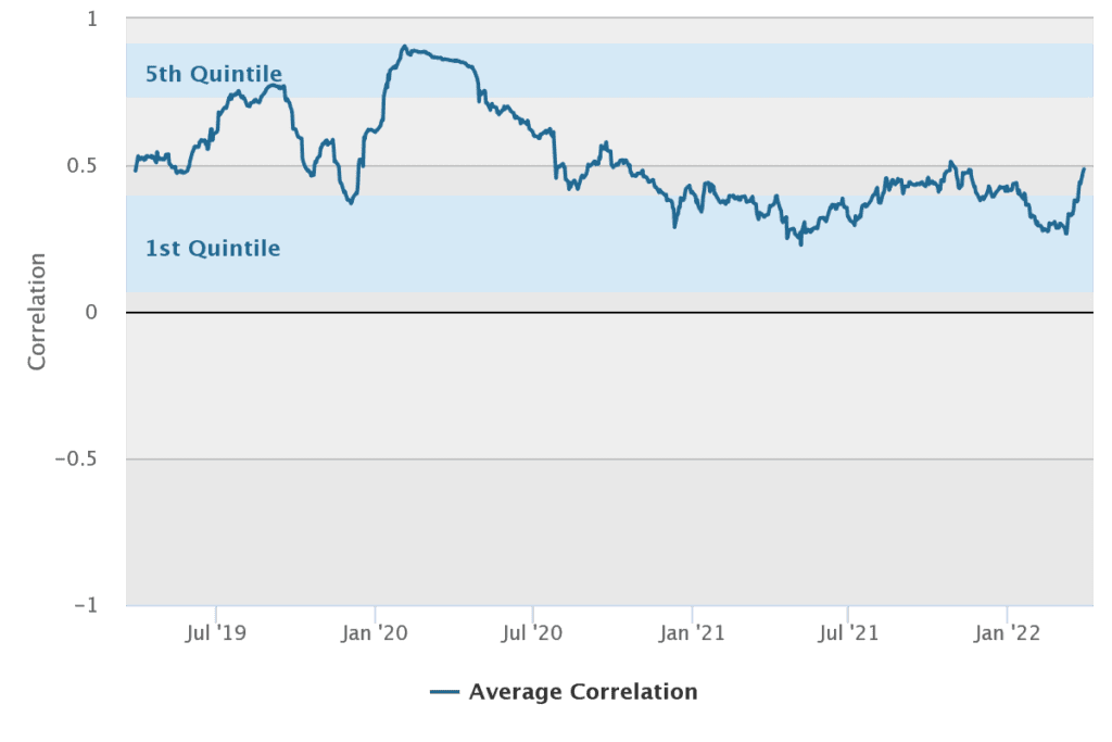
We also present Correlation Tables and Average Intra-Correlations from our Correlation Analysis product. Total Average Intra-Correlation is the average correlation of 4 constituents between them (6 correlations in total) in the whole equally-weighted portfolio.
The first multi-asset portfolio is constructed in a way to be lowly correlated between its constituents:
- US bonds with a 10-year maturity,
- US equities (publicly available data, for example, Fama & French offer free stock data with a long history),
- the selected basket of commodities,
- and finally US Dollar relative to other world currencies.
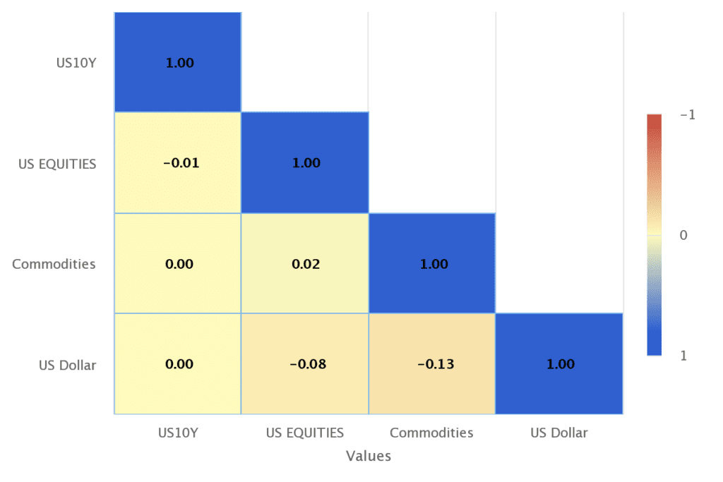
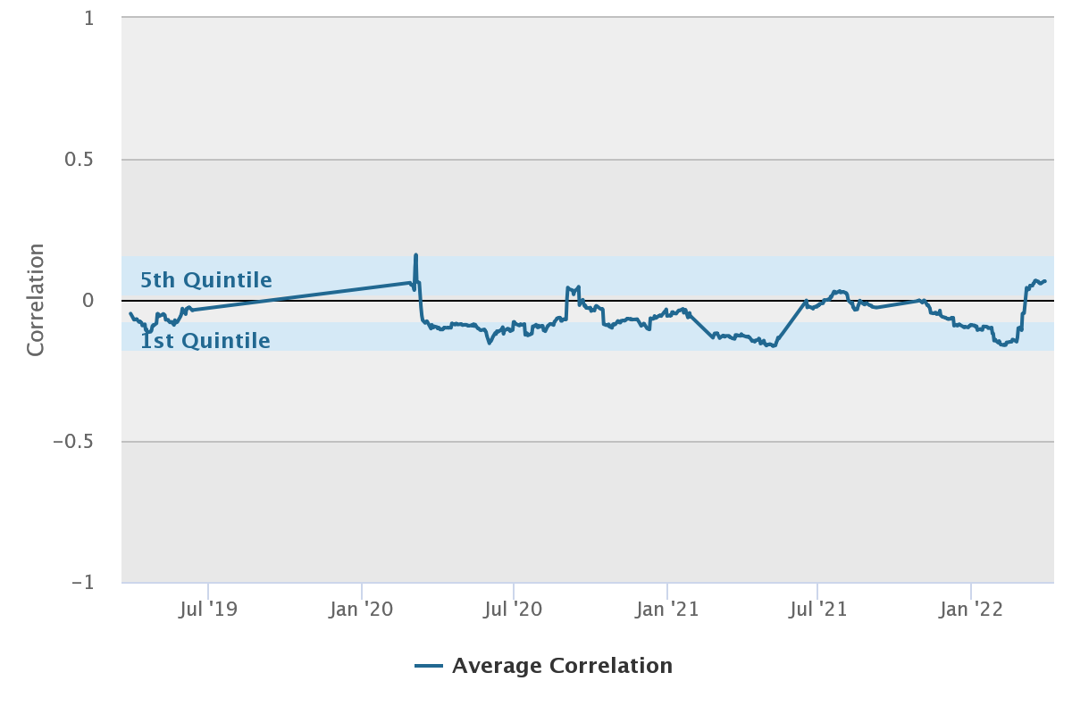
The total average correlation among constituents for portfolio #1 is -0.03, reflecting our goal of achieving a (very) low correlation between asset classes.
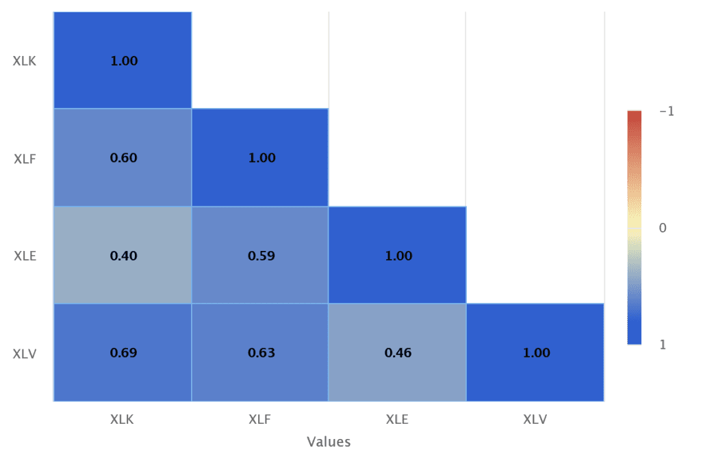
The second portfolio, on the other hand, is meant to be highly correlated and consists of US (markets sector) ETFs:
- XLK (Technology Select Sector SPDR Fund),
- XLF (Financial Select Sector SPDR Fund),
- XLE (Energy Select Sector SPDR Fund),
- XLV (Health Care Select Sector SPDR Fund).
We obtained historical data from Yahoo Finance and used close price adjusted for splits and dividend and/or capital gain distributions.
The total average correlation among constituents for portfolio #2 is 0.56, well in our intent to show the effects of high positive correlations on rebalancing processes.
Goals and Final Portfolios Construction
This report’s main goal is to determine the influence of rebalancing decisions on performance dispersion and suggest the optimal steps to achieve a steady rebalancing process.
We construct equally-weighted final portfolios (1/4 weight for each asset in either portfolios #1 or #2) that is initially allocated on 31/12/1999 with weights depending on performance from that day. The initial modeled investment is 100 USD. Following each relocation day, we reallocate accordingly, buying/selling the portion number of shares in the underlying from performance on that EOD. We do so until the end of our data sample, which is 31/03/2022.
Results
Our main focus is on showing the rebalancing performance dispersion, which we calculate as the difference between the highest and lowest performance in the selected subset of variants, divided by the average performance of that subsample.

Hypothesis #1: We assume that the lower the average correlation among constituents of the portfolio is, the higher the dispersion, in fact, is, making it better sense to look into various rebalancing options since it is more important to select the right rebalancing date to maximize potential profit and dampen volatility and drawdowns.
Portfolio #1:
Let’s now take a closer look at the long-time run of different best and worst variants of monthly and yearly rebalancing options for the first portfolio. The first table shows the performance and risk statistics of our portfolio when we rebalance monthly during different days in a month (for example -11 row shows results when we rebalance 11 days before the end of the month; on the other hand, +4 case means that we rebalance our portfolio at the end of the 4th day each month). The second table shows results for the portfolio that’s rebalanced once a month at the end of the different months.
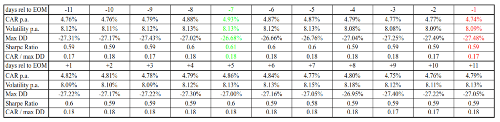
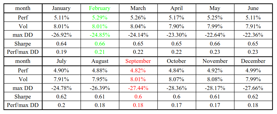
For a low-correlation portfolio, we get performance differences between monthly rebalances of 0.19% (the best case is 4.93% minus the worst case of 4.74%). The performance difference between the best and worst portfolios for the yearly rebalancing is 0.47% (5.29% – 4.82%). Now we can divide those numbers by the average performance over the monthly and yearly rebalancing periods (4.80% and 5.05%), which gives us performance dispersions of 3.95% (monthly rebalancing) and 9.32% (yearly rebalancing).
What do those numbers mean? The 9% dispersion in yearly performance due to rebalancing means that if we expect our portfolio to earn 10% a year, then rebalancing decisions can impact that final performance by 9% from the total performance, so 0.09*10% = 90bps. Our final performance can be anything between 9,55% and 10.45%, just due to rebalancing decisions. Is that too much? Is that not so much? It depends what’s your strategy. If you are not very active funds, then 9% relative dispersion just due to rebalancing can be significant. If you are a highly active fund, it can be something that is not so important. But we can’t judge this number in isolation with just one portfolio. Therefore we will soon look at the 2nd, more correlated portfolio to understand what’s the relative impact of rebalancing decisions among different portfolios.
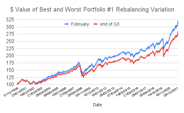
But before we move to the 2nd portfolio, let’s take a look at total performance dispersion using all the 43 rebalancing variants (all variants of daily, weekly, monthly, quarterly and yearly rebalancing): For portfolio #1, the best choice for rebalancing would be each February; on the other hand, the worst one if we take quarterly rebalances once per year and select end of Q3 (rebalance performed at the end of October). What’s the rebalancing dispersion? The difference between the best and the worst portfolio is 0.58% divided by average 4.87% makes total rebalancing dispersion 12%.
Portfolio #2:
Without a lot of words, let’s take a look at the tables that show the performance and risk characteristics for all variants of the second portfolio (more correlated) using different monthly and yearly rebalancing dates.
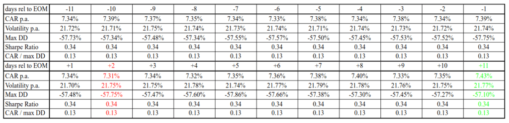
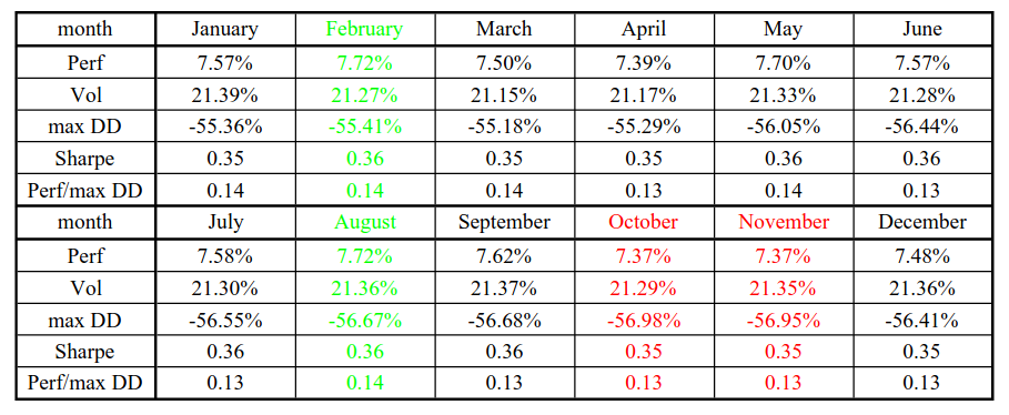
Data points of performance dispersions for the second, higher correlated portfolio for monthly rebalancing are 0.12% (7.43%-7.31%) divided by the average performance of 7.36% = 1.63%. In the case of yearly rebalancing, the performance dispersion is 0.35% (the spread in performance of 7.72% and 7.37%) divided by the average performance of 7.55% = 4.64%.
We can compare performance dispersion numbers between portfolios – a lowly correlated portfolio with a yearly rebalancing has a dispersion of 9.32%, and a highly correlated portfolio has a performance dispersion of 4.64%. We can clearly see that the effect of rebalancing is significantly more intensified in the less correlated portfolio.
What’s the total performance dispersion among all rebalancing variants?
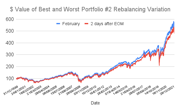
For portfolio #2, the worst choice would be to rebalance 2 days after the month turning (if monthly rebalance, once per month is selected), the best one in either February or August (if yearly, once per month is selected), the difference-making 0.41% divided by 7.43% results in total dispersion 6%, half compared to the lowly correlated portfolio.
Conclusion
We conclude that if we consider all of the variations, the distinction is apparent for both portfolios. Comparing all tested variants and considering all the presented results from both portfolios, we conclude that careful investors should consider rebalancing the dates of their portfolio since it can significantly affect the overall performance results. Especially, the dispersion in performance caused by different rebalancing strategies is increased mainly for the portfolios that are built from assets/strategies that have a low correlation.
Are you looking for more strategies to read about? Sign up for our newsletter or visit our Blog or Screener.
Do you want to learn more about Quantpedia Premium service? Check how Quantpedia works, our mission and Premium pricing offer.
Do you want to learn more about Quantpedia Pro service? Check its description, watch videos, review reporting capabilities and visit our pricing offer.
Do you want algorithmic access to the full Quantpedia database via the API? Subscribe to Quantpedia Pro, ask for an API key, and explore the in/out-of-sample statistics, source academic papers, and code snippets — ideal for quantitative research, systematic trading workflows, and AI model training.
Are you looking for historical data or backtesting platforms? Check our list of Algo Trading Discounts.
Or follow us on:
Facebook Group, Facebook Page, Telegram, Twitter, Linkedin, Medium or Youtube
Share onLinkedInTwitterFacebookRefer to a friend


