Most investors focus solely on the profitability of their investment strategy. And, even though having a profitable strategy is important, it is not everything. There are still numerous other things to consider. One of them is the size of the investment. The investment size can increase or decrease the profitability of a strategy, so it is essential to choose it right. The following article is our introduction to Kelly and Optimal F methodologies, that underlies our upcoming Quantpedia Pro report.
Introduction
There are various methods that focus on choosing the “correct” size of an investment. We already covered multiple position-sizing methods like Volatility Targeting or CPPI. In this article, we introduce another position sizing method – this time originally from trading and gambling environment.
First, we focus on a simple Kelly Criterion, which comes from theory of gambling. Later, we analyze a more advanced version called an Optimal f. And finally, as always, in the last section of this article, we demonstrate the theory on a specific investment strategy.
Kelly Criterion
John Larry Kelly Jr. is the author of the Kelly criterion formula from 1956. It was found that the formula, which has a gambling background and helps to determine the optimal bet size, can also help with finding the ideal investment size. The Kelly bet size is found by maximizing the expected geometric growth rate.
The simple version of the formula, which we use in the later section, is:
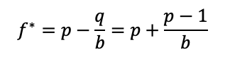
where f* is the optimal fraction, or in other words, the percentage of the total wealth that should be put at risk. On the left-hand side of the equation is:
p – the probability of a win
q – the probability of a loss (q=1-p), and
b – the amount gained with a win. So, for example, if we are betting on a 2-to-1 odds bet, then b=2.
The formula was originally designed for binary outcomes, such as coin flip, where you either win or lose. However, there is also a general form of the Kelly formula, which allows for partial losses. The partial losses are relevant for investments. This formula is:

here f* is the optimal fraction, or in other words, the percentage of the total wealth that should be put at risk. Next:
p is the probability that the investment increases in value
q is the probability that the investment decreases in value (q=1-p)
a is the fraction lost in a negative outcome and
b is the fraction gained in a positive outcome
For example, if the security price falls 10%, then a=0.1. On the other hand, if the security price rises 10%, then b=0.1.
In both of the abovementioned cases the f* falls between 0 and 1 by definition (if you have a profitable investment strategy, otherwise it may become negative).
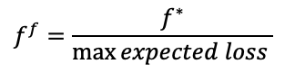
Finally, the common practice is to divide the fraction f* by the maximum expected loss of your strategy. This should result into your final position size. For example, if f*=0.2 and you expect a maximum loss of 10% on your strategy, then you should size your position as 0.2/10%=2 (leverage, i.e. 200% position size). If you expect a maximum loss of 100% is possible, then your optimal position size would be 0.2/100% = 20%.
Final “wager” scaling:
Optimal F
As we mentioned in the previous section, the basic Kelly formula was primarily designed for binary outcomes. In other words, you either win or lose, and the size of the win/loss is the same. However, in trading, we should expect our wins and losses to be of varying sizes. That’s when Optimal f comes into play. According to “Optimal f” by Ralph Vince the Optimal f calculates with the size of a trade and with the biggest loss from a set period. The formula for Optimal f is:
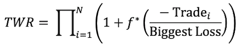
where we want to maximize the TWR, which stands for the Terminal Wealth Relative. So, we are looking for the f* that produces the highest TWR. Lastly, the Trade stands for the profit or loss on a trade, and the Biggest Loss is the Biggest Loss during a set period. In other words – the Optimal f formula stands for the maximization of the geometric average of your investment (relative to the biggest loss).
This method is much closer to the real-life optimal position sizing. However, it still tends to over-bet and use the leverage that is way too big. It is caused by the fact that the reality is usually worse than the backtest.
Similar to the Kelly formula, your final position size is then determined as f* divided by the biggest loss (or biggest expected loss). Once again, f* is bounded between 0 and 1 (if you have a profitable investment strategy, otherwise it may become negative). The final position size is then unbounded, because the leverage can be greater than one because it is measured against the maximal loss:
Backtest vs. Reality
As we probably all know from experience, the reality is oftentimes much worse than what we see in the backtests. That’s why we need to be cautious when deciding on the size of leverage. Research suggests that rather than thinking about Kelly as a goal, think about it as a boundary. So it is better to make the leverage smaller than what the Optimal f suggests.
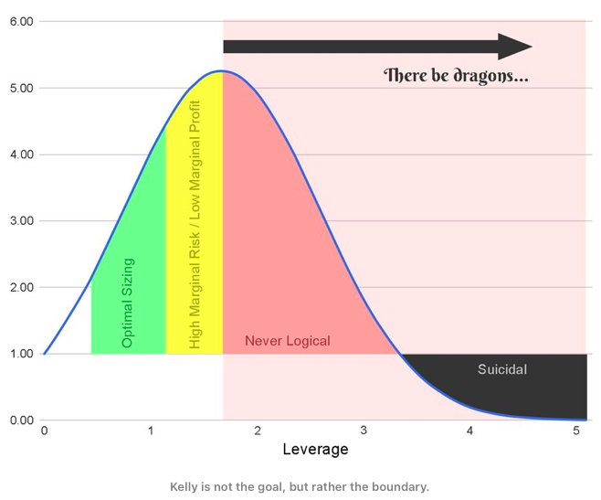
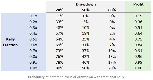
Looking at the figure above and the following table from an article by Yonder, 2021, we can see how the Kelly fraction affects the drawdown. For example, if we choose the Kelly Fraction = 1.0, then with the probability of 80%, we get a 20% drawdown; with the probability of 50%, we get a 50% drawdown; and with the probability of 20%, we get an 80% drawdown. Do you want to lose that much? No. That’s why it’s better to be a bit conservative and use just a fraction of the Kelly (or Optimal f).
There are various ways to pick this fraction (btw, here is a useful fraction calculator) and make sure we stay on the more conservative side, which is usually safer. The easiest way is to divide the Kelly f (/Optimal f) by maximal expected loss, which can either be estimated from the maximal loss from the previous period, or it can be fixed on a set level. Then it’s advised to downscale this number further – and bet/invest only a half or a third of it. These are rules of thumb. There are also several more sophisticated ways to deal with this problem.
Downscaling the optimal f* by bootstrap
The one of the more sophisticated ways of downscaling Optimal f we will demonstrate here is bootstrapping (sampling with replacement). To get a conservative assessment of the optimal position size/leverage we:
-perform 100 bootstraps from the strategy’s historical daily returns and then
-calculate the Kelly f (/Optimal f) from the 5th worst percentile (based on strategy performance) and finally we
-divide the Kelly f (/Optimal f) obtained this way by the maximum expected loss, as usually
Period returns or P&L of trades?
One technical, yet important question when talking about position sizing is – what kind of returns to use as inputs for further calculations? Should we use period returns (e.g. daily returns if the strategy trades daily) or trade returns? Daily returns mean roughly 250 data points each year, while trade returns will get you much less data points (given that you trade only on some days, not intraday).
Let’s say we have a strategy on a daily frequency which trades only once a month and holds the position for 5 days. Utilizing daily returns of the strategy, we will get a lot of “zeros” i.e. days when the strategy stays out of the market. On the other hand, utilizing trade returns, we will get 12 data points – each representing a P&L of a single trade.

Which option is better or more correct? That depends. There’s no correct answer. It’s just important to understand well what these numbers mean and interpret them correctly. We will demonstrate both options – “daily returns” as well as “trades”.
Investment Strategy
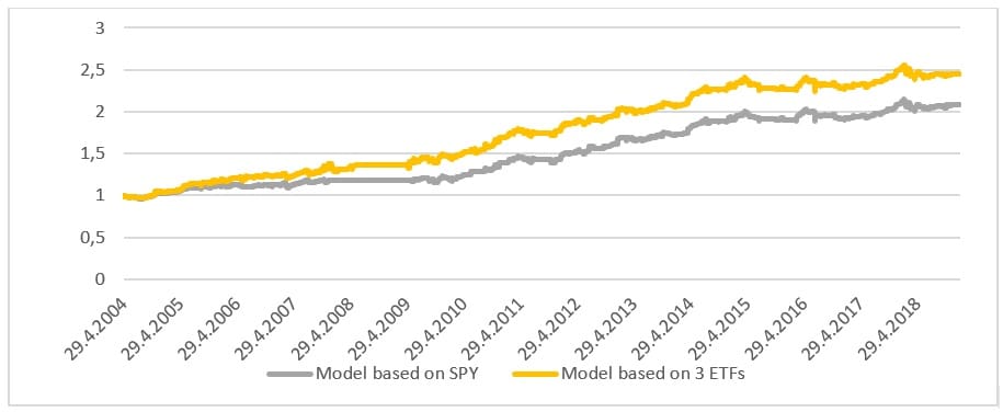
The strategy that we picked for this analysis is the Calendar / Seasonal Trading and Momentum Factor. This strategy is a combination of a simple profitable calendar strategies consisting of smaller blocks. The article above shows that momentum strategies combined with calendar anomaly rebalancing may result into a profitable strategy with attractive return to risk ratio. This strategy uses a diversified set of equity ETFs and is easy to replicate. It trades on a daily frequency and opens the trades only on given days. For more details about the strategy, please read the full blog post.
The equity curve of the strategy is depicted below:
| Would you like to test similar ideas yourself? Then, check exclusive discount offers for our readers for Historical Trading Data and Backtesting Platforms. |
Optimal position sizing – today, using entire history
We explore several approaches of calculating the optimal position sizing (leverages) for this strategy. We analyze a) the daily returns and b) the trade returns separately. Additionally, we calculate the Kelly f (/Optimal f) from a) the raw data, as well as b) the bootstrapped data.
By the bootstrapped data we mean 100 bootstraps as described above, and their 5th worst percentile. Here we calculated Kelly f (/Optimal f) from the bootstrapped data and divided it by the maximal expected loss, set to 10%. Additionally, we repeated this process with trades instead of daily returns. The maximal expected loss is set to 20% in this case.
If we wanted to start trading the strategy today, we could take the entire historical data of the strategy, calculate Kelly/Optimal f and then simply trade this amount of the strategy from now on. These are the optimal position sizing fractions of the 4 combinations described above:
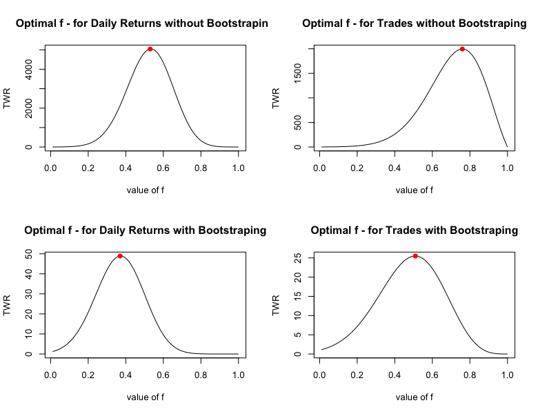
To arrive at the final position size, one must divide these numbers by their maximum expected loss (we chose 10% for daily returns and 20% for trades).
If we then apply this optimal position sizing to the historical returns of the strategy, it would look like the chart below

This, however, contains lookahead bias. We use the data from the past to calculate optimal position size which we then again apply to the same past data. To be entirely precise, we need to use only data available at the particular point in time. See next section.
Optimal Position sizing – historically, in time
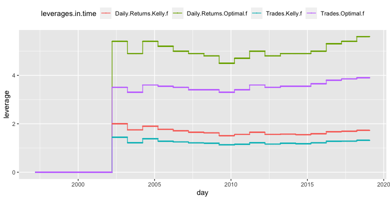
For daily returns – we started with the first five years of historical daily returns of the strategy and calculated the Kelly f and Optimal f from them. Then, we divided the Kelly f (/Optimal f) by the maximal expected loss to get the leverage. We set the maximal expected daily loss to 10%. Then, every year, we recalculate the new leverage from the whole data history available at that point in time (expanding window).
For trade returns – we repeated the same process with trades instead of daily returns. In this case, we set the maximum expected loss to 20%. The following figure shows the evolution of the 4 different optimal leverages we got from all four abovementioned methods.
Secondly, we applied our bootstrapping as described above. We started by calculating 100 bootstraps from the first five years of daily returns. Then we calculated the average return of each bootstrap and found the 5thworst percentile. After that, we calculated Kelly f (/Optimal f) from the bootstrapped data and divided it by the maximal expected loss, set to 10%. We then moved forward a year and followed with an additional year of data, etc. up to 2021. Additionally, we repeated this process with trades instead of daily returns. The maximal expected loss is 20% in this case. The following chart shows the obtained optimal leverages we got from all four methods using bootstrapping.

As we can see, the methods which calculate the Kelly f (/Optimal f) from bootstrapped data are more conservative and give us smaller leverages. Finally, we applied all of the calculated leverages to the daily returns at each point in time.
Leverage is not for free. Thus, we needed to take into consideration also leverage costs. We set the cost of leverage historically as 3M USD Libor + 2%.
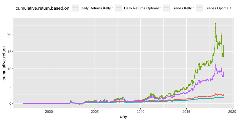
The following charts show the cumulative performance of such strategies. The first chart shows the cumulative returns of strategies calculated with leverages without bootstrap.
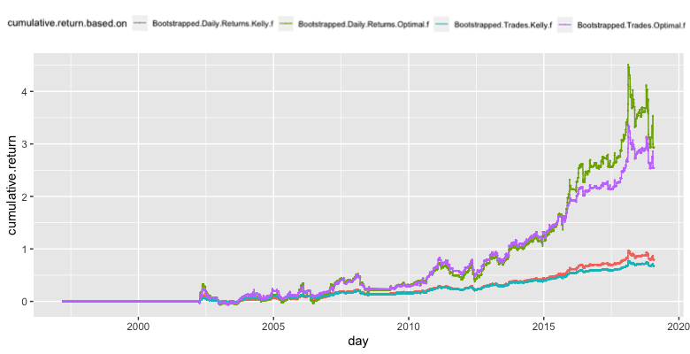
The second chart shows strategies, which are calculated using leverages from the bootstrapped data.
Lastly let’s take a look at the table of risk and return characteristics.

There’s no precise answer to the question which method is best to use. Rather than answering this question, this article aims for illustrating their differences. We may, however, observe several obvious tendencies among the data above.
Using 5th percentile of the bootstrap simulation results into considerably more conservative position sizing – roughly a half of that without bootstrapping. This is a desired property, though. The bootstrap was supposed to make our position sizing more conservative.
There’s no clear pattern on what works the best – whether Kelly or Optimal f, daily returns or trade returns. From the table above, it may seem as if using the trade returns resulted into more conservative position sizing. However, bear in mind that this is highly influenced by the maximum loss we expect (10% per day for daily returns, 20% per trade for trade returns) which is used in the denominator of the optimal size.
Another pattern which can be observed is that almost all of the position sizing methods achieved worse Sharpe ratio and Calmar ratio compared to the original strategy. However, if you think about it a bit more, this is to be expected – because of the leverage. Since the position sizing methods are using leverage (which is not for free), which harms return to risk ratios.
In our opinion, the position sizing which seems to be the most reasonable in this case out of the ones above is the Bootstrapped version of Optimal f (regardless of whether we calculate it for daily returns or trade returns). Mostly, due to its plausible logic, rather than superior results.
Author:
Daniela Hanicova, Quant Analyst, Quantpedia
Are you interested in more position sizing topics? Then look also at our Position Sizing course.
Are you looking for more strategies to read about? Sign up for our newsletter or visit our Blog or Screener.
Do you want to learn more about Quantpedia Premium service? Check how Quantpedia works, our mission and Premium pricing offer.
Do you want to learn more about Quantpedia Pro service? Check its description, watch videos, review reporting capabilities and visit our pricing offer.
Or follow us on:
Facebook Group, Facebook Page, Twitter, Linkedin, Medium or Youtube
Share onLinkedInTwitterFacebookRefer to a friend