Introduction to CPPI – Constant Proportion Portfolio Insurance
As we have promised, we present a short article as an introduction into the methodology of the Quantpedia Pro CPPI reports. Quantpedia Pro clients can use the model portfolio built in the Portfolio Manager as a risky asset to test various variants – Basic CPPI, Drawdown Based CPPI and Dynamic Multiplier CPPI.
Introduction
CPPI (Constant Proportion Portfolio Insurance) is a strategy that allows an investor to keep exposure to a risky asset’s upside potential while providing a guarantee against the downside risk by dynamically scaling the exposure. It’s a favourite strategy often used to build protected funds or as a part of various synthetic derivative products.
The main principle behind the CPPI strategies is not complicated at all. Imagine a portfolio consisting of two types of assets, “safe” (with a given yield y) and “risky”. Firstly, choose the protection level of the portfolio, i.e. the minimum value you want to protect (for example its starting value, s) and the protection period in years, T. It’s then easy to calculate how much may the portfolio value decline at each point in time t, so that the safe asset will be able to recover the loss back to the protection level:
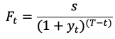
This is the floor (the value, you don’t want to go below). The difference between the current portfolio value and the floor is then called cushion; it is the value you can put at risk.
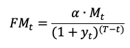
At every point in time, you can allocate multiplier M of the cushion to the risky assets. Thus, as the cushion decreases, you are reducing the risky asset allocation. If the cushion goes to zero (the value of the portfolio hits the floor), your allocation to the risky assets is the multiplier M times zero. This means you are allocating nothing to the portfolio’s risky portion, and 100% is invested in the safe component of your portfolio.

CPPI procedure creates convex option-like payoffs without actually using options. The most significant benefit of CPPI strategy is that if you were able to trade continuously, nothing could go wrong. However, we have to take into an account the transaction costs and the gap risk. Because transaction costs go up the more often you trade, you may want to trade on a less frequent basis, e.g. monthly. However, this creates an opportunity for things to go wrong.
The loss of the risky component can become large enough that you get below the floor between two trading dates. The risk of breaching the floor this way is called “the gap risk”. That gap risk materializes if and only if the loss on the risky asset exceeds 1/M within the trading interval. Because of this, it is recommended to set the multiplier as a function of the maximum potential loss within a given trading interval.
Extension models
Maximum Drawdown Extension
There are a few extension models one can use to improve their CPPI strategy. The first one we introduce is the Maximum Drawdown extension. This method sets the protection level as a predefined percentage loss from the peak value of the portfolio. This loss from the peak is given by the maximum drawdown. The idea lies in keeping the maximum drawdown at the end of the protection period below a set limit.
For example, let the maximum acceptable drawdown at the end of the protection period be 20%. Then the value of portfolio at the end of the protection period has to be greater than a = 80% of the highest value the portfolio has ever reached ![]() :
:
![]()
At each time t, before the protection period the similar equation holds for the maximum drawdown floor calculation:
If maximum acceptable drawdown is set to 0%, i.e. a = 100%, the method essentially protects every new maximum the portfolio has achieved.
Cap Extension
The second extension of the CPPI on top of the floor (which you do not want to get under) also includes a cap, which you do not want to get over with your risky asset exposure. The cap is used because by giving up potential gains, an investor can protect potential loses. In practice, it is done by defining a threshold level ![]() at time t. The threshold level’s upper bound is the cap at time t, and the lower bound is the floor
at time t. The threshold level’s upper bound is the cap at time t, and the lower bound is the floor ![]() at time t:
at time t:
![]()
Suppose the portfolio value at time is between the floor value and the threshold value, to avoid hitting the floor. In that case, an investor allocates to the risky asset ![]() the multiplier M times the difference between the portfolio value ant the floor value (the cushion):
the multiplier M times the difference between the portfolio value ant the floor value (the cushion):
![]()
On the other hand, if the asset value ![]() at time is between the threshold value and the cap value, to avoid hitting the cap, an investor allocates to the risky asset the multiplier M times the difference between the cap value ant the portfolio value:
at time is between the threshold value and the cap value, to avoid hitting the cap, an investor allocates to the risky asset the multiplier M times the difference between the cap value ant the portfolio value:
![]()
The remaining question is how to find the threshold value. The threshold value is obtained by imposing the “smooth-pasting” condition. If the portfolio value is equal to the threshold value, the allocation to the risky asset can be written in two equal ways:
![]()
From this equation, we get a pretty simple answer. The threshold value is the average of the floor value and the cap value:
![]()
CPPI in practice
As we discussed in the previous part, CPPI is a strategy that protects investors’ portfolio against the downside risk while keeping exposure to the risky asset’s upside potential. We decided to take a closer look at a few CPPI models. To make our analysis realistic, we used SPY ETF as our risky asset and the United States 2-Year Bond Yield as our safe asset. Using the 2-Year Bond Yield means our floor is not linear in time, because it varies with changes in bond yields. Additionally, we used a 2-day lag in our calculations, which in combination with the non-linear floor and equity gap risk, leads to occasional minor breaches of the floor value.
We conducted two types of analysis. In both cases, we decided to analyze 5-year periods. The first one is a single period analysis. In the single period analysis, we firstly analyze the CPPI performance and floor evolution during one specific five-year period. Secondly, we present a table that compares the risk characteristic of the pure SPY portfolio and the CPPI portfolio.
In the second analysis we conduct a simulation of multiple 5-year periods, each starting one month after the start of the previous one. We decided to perform this multi-period simulation to robustly evaluate how the CPPI behaves in the long run. The first period started in January 2006, and the last one starts in January 2016, which gives us 120 five-year periods. This way we obtain a distribution of different CPPI paths, which we can analyze further. We compare the CPPI results with SPY and we provide charts of the 5-year annualized cumulative returns, Sharpe Ratios and maximum drawdowns, as well as tables that compare risk characteristics of both CPPI distribution and SPY distribution.
In general, CPPI does not beat a pure SPY portfolio in terms of performance because stocks perform well in the long run. Also, the Sharpe ratio may not improve when using CPPI. However, the main benefits of CPPI are on the risk side – the protection of the capital and much lower drawdowns and volatilities.
BASIC CPPI
The first model we introduce and which we call the “basic CPPI” protects the starting value of the portfolio. This means that if a portfolio’s initial value is, for example, $100 at the start of the 5-year period, the value will be at least $100 at the end of the period.
In the first example, we examined the 5-year period starting in January 2007. The table below shows the risk characteristics of the Basic CPPI portfolio compared to the pure SPY portfolio.
|
|
5Y CAR |
5Y Volatility |
Sharpe |
Max DD |
95% DD |
CAR/ |
CAR/ |
|
Basic CPPI |
-0.09% |
7.02% |
-0.013 |
-14.55% |
-14.01% |
0.006 |
0.007 |
|
SPY |
-0.91% |
26.49% |
-0.034 |
-55.19% |
-44.28% |
0.016 |
0.020 |
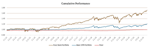
The following figure shows the cumulative performance of the Basic CPPI portfolio and pure SPY portfolio, as well as evolution of the floor in time.

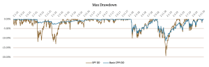
The chart above shows that the Basic CPPI portfolio hit the floor in October 2008, but it managed to outperform the pure SPY portfolio. The next figure shows the drawdowns of both of these portfolios.
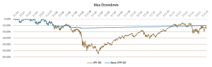
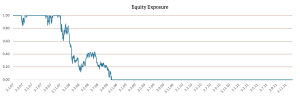
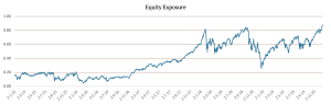
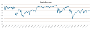
We can see that SPY’s drawdown is much greater than the basic CPPI portfolio drawdown, which is the most significant benefit of using the CPPI strategy. The following figure shows the equity exposure during the 5-year period.
The second example we introduce is the 5-year period starting in January 2015. The table below shows the risk characteristics of the Basic CPPI portfolio compared to the pure SPY portfolio.
|
|
5Y CAR |
5Y Volatility |
Sharpe |
Max DD |
95% DD |
CAR/ |
CAR/ |
|
Basic CPPI |
3.92% |
5.81% |
0.676 |
-11.55% |
-6.42% |
0.340 |
0.611 |
|
SPY |
11.39% |
13.41% |
0.849 |
-19.35% |
-9.22% |
0.588 |
1.235 |
The following figure shows the cumulative performance of the Basic CPPI portfolio and pure SPY portfolio, as well as the floor development.
In this case, the Basic CPPI portfolio did not outperform the pure SPY portfolio. However, as we can see in the next figure, the Basic CPPI portfolio drawdowns were much lower compared to the SPY’s drawdowns.
The last figure shows the equity exposure during the 5-year period from January 2015.
Drawdown-based CPPI
Another model we introduce is a drawdown-based CPPI. The main idea behind this model is to protect a certain drawdown level. In other words, loss on the CPPI portfolio at the end of the protection period should not be greater than the pre-specified drawdown level. Once again, we present two examples of this model. In the first example, we protect 10% drawdown. The following table shows the risk characteristics of the 10% Drawdown CPPI portfolio and the pure SPY portfolio.
|
|
5Y CAR |
5Y Volatility |
Sharpe |
Max DD |
95% DD |
CAR/ |
CAR/ |
|
10% Drawdown CPPI |
5.19% |
6.29% |
0.826 |
-8.78% |
-6.31% |
0.591 |
0.823 |
|
SPY |
11.39% |
13.41% |
0.849 |
-19.35% |
-9.22% |
0.588 |
1.235 |
As we can see, the SPY portfolio did outperform the 10% Drawdown CPPI portfolio. However, the SPY’s drawdown is more than twice greater than the 10% Drawdown CPPI portfolio’s drawdown and both the Sharpe ratio and the Calmar ratio are almost identical. The figure below shows the cumulative performance of both portfolios and the floor.

The next figure compares the drawdowns of the 10% Drawdown CPPI portfolio and the pure SPY portfolio.
As we can see, the drawdowns were significantly lower when using a 10% Drawdown CPPI portfolio compared to SPY. The figure below shows the equity exposure during the 5-year period from January 2015.
The second example we present is the “New High CPPI”, which can be explained as a 0% drawdown protection level. This means that each time the performance reaches a new high, CPPI locks and protects this value until the end of the 5-year period. The New High CPPI portfolio’s risk characteristics and the pure SPY portfolio are presented in the table below.
|
|
5Y CAR |
5Y Volatility |
Sharpe |
Max DD |
95% DD |
CAR/ |
CAR/ |
|
New High CPPI |
1.99% |
1.49% |
1.338 |
-2.12% |
-1.48% |
0.936 |
1.341 |
|
SPY |
11.39% |
13.41% |
0.849 |
-19.35% |
-9.22% |
0.588 |
1.235 |
The table shows that even though the SPY portfolio did outperform the New High CPPI portfolio significantly, the Sharpe Ratio of the New High CPPI portfolio is much greater. This is a consequence of a very defensive nature of this model. Naturally, also the maximum drawdown is significantly better when using the New High CPPI strategy. The figure below shows the cumulative performance of both portfolios and the floor.
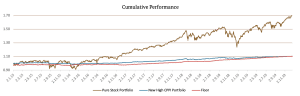
This figure shows that the New High CPPI portfolio hit the floor right at the end of our 5-year period, although it moved close to it for the entire period under inspection. The next figure shows the drawdowns of the New High CPPI portfolio and the pure SPY portfolio.
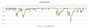
As we can see, the drawdowns are minor when using the New High Drawdown CPPI portfolio. The next figure shows the equity exposure during the 5-year period from January 2015.
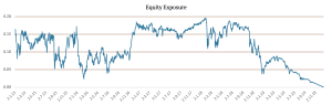
Here we can observe the typical behavior of the New High CPPI, which always gradually decreases the risk towards end of the 5-year horizon. As you can see, the New High CPPI is an extremely conservative variant with very low average exposure to risky assets.
Dynamic Multiplier CPPI
The last method we examine is a Dynamic Multiplier CPPI. In the previous methods, we use a fixed multiplier of 5. However, in this one, we change the multiplier based on the volatility of SPY. In times of a high volatility we lower the multiplier and vice versa in times of a low volatility.
We calculate a 21-day EWMA volatility and a 63-day simple volatility and compare each one with their 126-day moving average. Then we set our conditions: if both of the volatilities were above their respectful moving average during the past three days, we use the multiplier of 2; if both of the volatilities were below their respectful moving average during the past three days, we use the multiplier of 8; otherwise, we use the default multiplier of 5.
The following table shows the risk characteristics of this CPPI method compared to the Basic CPPI and pure SPY portfolio.
|
|
5Y CAR |
5Y Volatility |
Sharpe |
Max DD |
95% DD |
CAR/ |
CAR/ |
|
Basic CPPI |
3.92% |
5.81% |
0.676 |
-11.55% |
-6.42% |
0.340 |
0.611 |
|
Dynamic Multiplier CPPI |
4.37% |
5.49% |
0.795 |
-10.33% |
-7.26% |
0.423 |
0.601 |
|
SPY |
11.39% |
13.41% |
0.849 |
-19.35% |
-9.22% |
0.588 |
1.235 |
We can see that the Dynamic Multiplier CPPI portfolio has slightly better performance and Sharpe Ratio compared to the Basic CPPI portfolio.
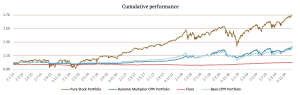
The figure above shows the cumulative performance of the SPY portfolio, Basic CPPI portfolio, Dynamic Multiplier CPPI portfolio and the changing floor. As we can once again see, the drawdowns of the Dynamic Multiplier CPPI portfolio are much lower compared to the SPY’s drawdowns. This is better illustrated in the figure below.
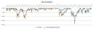
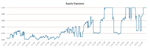
The last figure shows the Dynamic Multiplier CPPI portfolio’s equity exposure during the 5-year period from January 2015. Jumps are to be expected due to dynamic changes in the multiplier.
Simulations
As we mentioned at the beginning of this article, we conducted two types of analysis. In this part, we present the simulations of multiple 5-year periods, each starting one month after the start of the previous one. The first period began in January 2006, and the last one begins in January 2016, which gives us 120 five-year periods. We then compare the results of the distribution we obtain of the CPPI vs. SPY and show distribution charts of the 5-year annualized cumulative returns, Sharpe Ratios and maximum drawdowns, as well as tables that compare distributions of risk characteristics of CPPI and SPY portfolios.
Firstly, we present the resulting table for the pure SPY portfolio. The first row represents the 5th percentile of the simulations, the second row gives the median result, and the last row presents the 95th percentile out of all the simulations.
|
|
Results of SPY simulation |
||||||
|
5Y CAR |
5Y Volatility |
Sharpe |
Max DD |
95% DD |
CAR/ |
CAR/ |
|
|
5th percentile |
0.00% |
12.15% |
0.00 |
-55.19% |
-44.28% |
0.01 |
0.02 |
|
median |
11.86% |
15.76% |
0.81 |
-19.35% |
-11.21% |
0.60 |
1.21 |
|
95th percentile |
17.38% |
26.48% |
1.21 |
-13.02% |
-7.01% |
1.16 |
2.12 |
BASIC CPPI
Once again, we start with the Basic CPPI, where we protect the portfolio’s starting value. The table below shows the results for the Basic CPPI portfolio simulations.
|
|
Results of Basic CPPI simulation |
||||||
|
5Y CAR |
5Y Volatility |
Sharpe |
Max DD |
95% DD |
CAR/ |
CAR/ |
|
|
5th percentile |
-0.10% |
2.31% |
-0.03 |
-22.91% |
-20.78% |
0.00 |
0.00 |
|
median |
2.46% |
4.92% |
0.50 |
-9.12% |
-5.93% |
0.27 |
0.46 |
|
95th percentile |
7.62% |
11.73% |
1.01 |
-3.76% |
-2.62% |
0.91 |
1.36 |
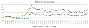
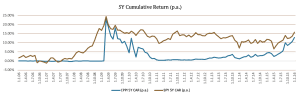
When we compare the simulations of Basic CPPI and the pure SPY, we can see that even though the 5-year CAR of the Basic CPPI strategy is lower, this strategy confirmed its role in lowering volatilities and drawdowns. The following figure compares the 5-year annualized cumulative returns of the Basic CPPI strategy and SPY. The dates on the X-axis represent the starting day of the 5-year period.
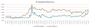
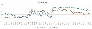
We can see that the return of the SPY portfolio is much better in almost every 5-year period. However, there are a few periods at the beginning where the Basic CPPI outperformed the SPY portfolio (crisis of 2008). The next figure shows the Sharpe Ratios of the simulations.
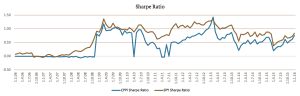
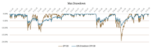
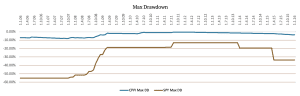
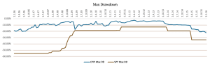
This chart shows that even though there are significant differences in the returns, the Sharpe Ratios are not that different, which means the volatility is much lower when using Basic CPPI. Lastly, the figure below represents the maximum drawdowns during all the 5-year periods.
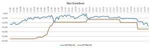
The maximum drawdowns are visibly lower in the simulations from January 2006 till January 2009 when using Basic CPPI.
Drawdown-based CPPI
Secondly, we simulated the drawdown-based CPPI model. Once again, we protect the 10% drawdown. We present the results in the same manner as the ones before:
|
|
Results of 10% Drawdown CPPI simulation |
||||||
|
5Y CAR |
5Y Volatility |
Sharpe |
Max DD |
95% DD |
CAR/ |
CAR/ |
|
|
5th percentile |
-1.77% |
4.90% |
-0.39 |
-15.68% |
-15.09% |
0.03 |
0.03 |
|
median |
4.92% |
6.07% |
0.77 |
-8.18% |
-6.42% |
0.57 |
0.79 |
|
95th percentile |
6.91% |
7.79% |
1.13 |
-6.73% |
-4.69% |
0.93 |
1.32 |

New High CPPI
Another version of the drawdown-based CPPI model is the New High CPPI. This model allows the portfolio value to fall only to such extent, that it will reach its maximum value till the end of the period again. We present the results in the same manner as the ones before:
|
|
Results of New High CPPI simulation |
||||||
|
5Y CAR |
5Y Volatility |
Sharpe |
Max DD |
95% DD |
CAR/ |
CAR/ |
|
|
5th percentile |
0.02% |
0.53% |
0.02 |
-7.57% |
-6.93% |
0.01 |
0.01 |
|
median |
1.00% |
1.28% |
0.77 |
-2.03% |
-1.59% |
0.58 |
0.74 |
|
95th percentile |
3.13% |
5.17% |
1.62 |
-0.55% |
-0.37% |
1.55 |
2.24 |

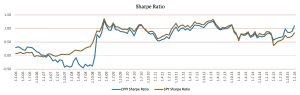
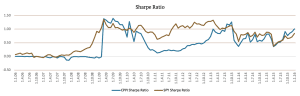
This chart shows that even though there are significant differences in the returns, the Sharpe Ratios are not that different. Additionally, since August 2011 the New High CPPI portfolio showed higher Sharpe Ratios.
Dynamic Multiplier CPPI
The last method we examine is the Dynamic Multiplier CPPI. As we already explained in this article, the previous methods use a fixed multiplier of 5. However, this one changes the multiplier based on the volatility of SPY. We present the results in the same manner as the ones before:
|
|
Results of Dynamic Multiplier CPPI simulation |
||||||
|
5Y CAR |
5Y Volatility |
Sharpe |
Max DD |
95% DD |
CAR/ |
CAR/ |
|
|
5th percentile |
-0.14% |
1.63% |
-0.05 |
-19.97% |
-17.39% |
-0.01 |
-0.01 |
|
median |
1.15% |
3.47% |
0.44 |
-9.05% |
-6.22% |
0.20 |
0.29 |
|
95th percentile |
12.20% |
11.17% |
1.26 |
-3.39% |
-2.81% |
1.26 |
2.14 |
Author:
Daniela Hanicova, Quant Analyst, Quantpedia
Side note – if you are interested in more position sizing methods, do not miss a new practically oriented course called Position Sizing in Trading, which we have launched with cooperation with QuantInsti and which aims to explain the money management techniques to intermediate level traders. The course presents an Index Reversal trading strategy written in python and applies to it different position sizing methods like Kelly Criterion, Optimal F, CPPI (Constant Proportion Portfolio Insurance), TIPP (Time-Invariant Protected Portfolio) and Volatility Targeting. Additionally, the course shows how to deal with performance deterioration, non-stationarity and fat-tails in the financial markets so that you have a complete conservative framework for position sizing. You are sincerely invited to visit the course’s introductory page (plus, you may apply for a 65% discount during the launching period until the 11th of July) …
Are you looking for more strategies to read about? Sign up for our newsletter or visit our Blog or Screener.
Do you want to learn more about Quantpedia Premium service? Check how Quantpedia works, our mission and Premium pricing offer.
Do you want to learn more about Quantpedia Pro service? Check its description, watch videos, review reporting capabilities and visit our pricing offer.
Do you want algorithmic access to the full Quantpedia database via the API? Subscribe to Quantpedia Pro, ask for an API key, and explore the in/out-of-sample statistics, source academic papers, and code snippets — ideal for quantitative research, systematic trading workflows, and AI model training.
Are you looking for historical data or backtesting platforms? Check our list of Algo Trading Discounts.
Or follow us on:
Facebook Group, Facebook Page, Telegram, Twitter, Linkedin, Medium or Youtube
Share onLinkedInTwitterFacebookRefer to a friend


