Bitcoin ETFs in Conventional Multi-Asset Portfolios
Understanding how Bitcoin-related instruments can fit into traditional portfolios is increasingly relevant for investors. Some risk-averse investors do not like to hold cryptocurrencies in their portfolios strategically; however, they may be open to investing in crypto-linked assets on a tactical level. In this context, our goal is to explore how we can provide short-term Bitcoin exposure while contributing to overall portfolio balance and potential downside protection.
Basic strategy – 10-day high Bitcoin strategy
The 10-day high strategy for Bitcoin is a momentum-based trading approach that assumes assets reaching new local highs are likely to continue their short-term trend. The strategy works as follows:
Our earlier Quantpedia research shows that a 10-day lookback window provides effective balance for momentum strategies in Bitcoin. In Revisiting Trend-Following and Mean-Reversion Strategies in Bitcoin, shorter windows such as 10 days delivered stronger and more robust risk-adjusted returns than longer horizons. Moreover, as highlighted in How to Profitably Trade Bitcoin’s Overnight Sessions, Bitcoin’s behavior differs across intraday and overnight cycles; a 10-day window naturally incorporates several such cycles, smoothing out session-specific anomalies while remaining responsive to fast-changing market dynamics.
Entering a position at a 10-day high is advantageous for a trend-following approach because it builds on existing momentum. When Bitcoin (ETF) breaks through a short-term local maximum, it often attracts additional buying interest and signals the continuation of the trend. A 10-day window is short enough to capture new moves quickly while still long enough to filter out random noise, making it an effective balance for identifying meaningful price momentum.
Data & assets
We based our analysis on daily close data from January 2018 through May 30, 2025, focusing on four representative exchange-traded funds.
BITO serves as an ETF vehicle for Bitcoin exposure through regulated futures, making it one of the most accessible instruments for investors seeking crypto allocation in traditional markets. For the period from 2018 until BITO’s launch in 2021, we synthetically reconstructed its historical performance using Bitcoin futures, as there were no U.S.-listed ETFs or similarly standardized assets available. We deliberately limited the historical window prior to 2018 because Bitcoin trading was largely confined to spot exchanges that suffered from fragmented liquidity, limited regulatory oversight, high volatility, and notable counterparty risks. These conditions reduced the reliability and practical relevance of empirical results for institutional-style portfolio construction, making earlier data less suitable for (robust) backtesting. In spring 2024, numerous new Bitcoin spot ETFs appeared, such as IBIT, FBTC, or GBTC. Now, it’s easy to access the spot Bitcoin market; however, for our historical analysis, we use the futures and futures ETF as it provides a longer historical window over which we can run our tests.
Among other ETFs we use: GLD tracks the price of gold and represents the traditional safe-haven asset in times of market stress. IEF holds intermediate-term U.S. Treasury bonds, a classic fixed-income component often associated with the defensive, risk-off side of portfolios. Finally, SPY mirrors the S&P 500 index and acts as a broad proxy for U.S. equities.
Benchmarks
To evaluate the potential contribution of these assets to a diversified portfolio, we aimed to construct an in-sample, Sharpe ratio–optimized portfolio with fixed allocations. This approach allowed us to identify portfolios that maximize expected return per unit of volatility within the sample period, providing a clear benchmark for how Bitcoin exposure via BITO interacts with traditional assets. Using the Sharpe ratio as the optimization criterion ensures that both risk and return are considered, highlighting combinations that are efficient from a risk-adjusted perspective.
Constructing a Markowitz-style portfolio without BITO results in an allocation of approximately 64.31% in GLD and 35.69% in SPY. When a fixed allocation to BITO is included, the optimal portfolio shifts to roughly 60% GLD, 30% SPY, and 10% BITO.
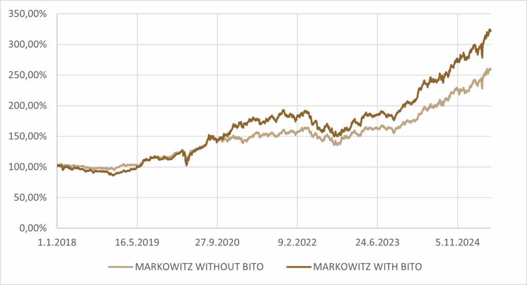
Table 1: Performance metrics of Markowitz Sharpe-ratio optimized portfolios.
| PORTFOLIO | CAR p.a. | VOL p.a. | SHARPE |
|---|---|---|---|
| Markowitz optimal with BITO | 17.06% | 13.44% | 1.27 |
| Markowitz optimal without BITO | 13.69% | 12.40% | 1.10 |
Bonds, represented here by IEF, proved less attractive for inclusion during the period under study. High inflationary pressures between 2022 and 2024 led to weak bond performance, limiting their ability to stabilize the portfolio. From a Sharpe ratio perspective, allocating to IEF contributed little to risk-adjusted returns, which is why the optimal portfolio excluded it entirely.
In contrast, gold experienced a significant bull market during the same period. This strong performance increased the expected return contribution of gold, boosting the portfolio’s Sharpe ratio. As a result, gold naturally became the dominant component of the optimized allocation, alongside SPY, to maximize expected return per unit of volatility.
It is important to note that constructing the portfolio based on in-sample Sharpe ratio optimization is definitely not the ideal allocation for future periods. Market conditions, volatility, and asset correlations can change, meaning that allocations derived from these historical data are not necessarily representative of long-term optimal allocations, as the specific conditions that favored gold, limited bond performance, and shaped correlations among assets during this period may not recur in the future. This portfolio should therefore be used primarily as a comparative benchmark for the sample period rather than a definitive guide for long-term allocation.
Bitcoin exposure via BITO is limited to roughly 10% of the portfolio because, despite its high expected returns, it also exhibits substantial volatility. Even a modest allocation can significantly increase overall portfolio risk. From a Sharpe ratio perspective, the 10% allocation represents a balance between capturing potential upside and avoiding excessive risk. In fact, for some investors or under slightly different market conditions, even this 10% could be considered aggressive, highlighting the importance of carefully assessing risk tolerance when incorporating highly volatile assets like BITO.
As an additional point of comparison, we will primarily use a simple 60/40 allocation between SPY and IEF as a reference benchmark. This traditional mix reflects a balanced approach between equities and bonds, capturing growth potential while providing stability through fixed-income exposure. Using this benchmark allows us to evaluate the incremental impact of including BITO or other deviations from a straightforward, historically grounded allocation.

Table 2: Performance metrics of 60% SPY & 40% IEF portfolio.
| PORTFOLIO | CAR p.a. | VOL p.a. | SHARPE |
|---|---|---|---|
| 60% SPY & 40% IEF | 8.54% | 11.96% | 0.71 |
Risk-on & risk off
Rather than relying solely on fixed portfolio weights, we want to shift toward a two-regime allocation framework that distinguishes between “risk-on” and “risk-off” environments. In a risk-on regime, market conditions for cryptocurrencies are favorable, and investors are more willing to take exposure to higher-volatility assets such as Bitcoin. Conversely, in a risk-off regime, risk appetite declines, and capital tends to flow into more defensive or lower-volatility assets. To operationalize this regime shift, we will use a 10-day high indicator for BITO. The strategy works as follows:
Here, we focus on our first portfolio—the risk-on portfolio. This portfolio follows a trend-following strategy, aiming to capitalize on upward movements in BITO. The approach is to maintain a long position as long as the asset continues to exhibit a positive trend, thereby capturing potential gains while the market remains favorable. The risk-on portfolio is fully fixed, with constant asset weights throughout the period.
The risk-off portfolio is a defensive portfolio, maintaining fixed asset weights throughout the period.
First iteration – From benchmark to BITO allocations
If we focus solely on BITO and disregard other assets, we can test the effectiveness of our 10-day high strategy. Following the process described above, the risk-on approach implies allocating 100% of the portfolio to BITO, while in the risk-off regime, the portfolio remains entirely in cash (with 0% yield, for the simplicity).

Table 3: Performance metrics of 100% BITO for 10-day high portfolio.
| PORTFOLIO | CAR p.a. | VOL p.a. | SHARPE |
|---|---|---|---|
| 100% BITO 10-day high | 23.23% | 36.49% | 0.64 |
The backtest results suggest that this strategy is relatively reliable, which provides a basis for constructing a pair of portfolios that can be alternated depending on market conditions. We take as a starting point one of the benchmark allocations introduced earlier, the 60% SPY and 40% IEF portfolio, and treat it as our risk-off portfolio. To create the corresponding risk-on portfolio, we reallocate 10 percent of the total weight to BITO, reducing the SPY and IEF positions proportionally. This adjustment results in a composition of 54% SPY, 36% IEF, and 10% BITO. Results of this approach are:


Table 4: Performance metrics of risk-on, risk-off, benchmark and 10-day high signal strategy portfolios.
| PORTFOLIO | CAR p.a. | VOL p.a. | SHARPE |
|---|---|---|---|
| Benchmark (60% SPY, 40% IEF) | 8.54% | 11.96% | 0.71 |
| 10-day high signal strategy (risk-on/off switch) | 10.54% | 12.50% | 0.84 |
| Risk-on (54% SPY, 36% IEF, 10% BITO) | 12.44% | 13.35% | 0.93 |
| Risk-off (60% SPY, 40% IEF) | 8.54% | 11.96% | 0.71 |
Compared to the 60/40 benchmark, the 10-day high strategy improved performance both in absolute and risk-adjusted terms. The Sharpe ratio rose from 0.71 to 0.84, reflecting higher returns with only a modest increase in volatility. Having the Bitcoin whole time (Risk-on) offered higher performance and Sharpe ratio; on the other hand, not all investors are comfortable with strategic allocation for cryptocurrencies, and tactical switching can be better in this case.
Second iteration – From IEF to GLD
The benchmark portfolio of 60% SPY and 40% IEF was not particularly well suited for the observed period, as its performance was relatively weak. This was driven largely by the underperformance of bonds, which limited the overall risk-adjusted return of the portfolio. It would therefore be reasonable to reallocate a portion of the benchmark into alternative assets. In our case, we introduce a 10 percent allocation to GLD, which provides diversification benefits and better aligns with the strong performance of gold during this period. Building on this adjustment, we use the revised benchmark with a 10 percent allocation to GLD as the risk-off portfolio and adjust the risk-on portfolio in a similar manner.

This adjustment results in a set of newly defined portfolios, each reflecting a different regime and allocation structure. By introducing GLD into the benchmark and applying the risk-on/risk-off framework, we obtain the following portfolios with their respective performance metrics:


Table 5: Performance metrics of risk-on, risk-off, benchmark and 10-day high signal strategy portfolios.
| PORTFOLIO | CAR p.a. | VOL p.a. | SHARPE |
|---|---|---|---|
| Benchmark (54% SPY, 36% IEF, 10% GLD) | 9.12% | 11.13% | 0.82 |
| 10-day high signal strategy (risk-on/off switch) | 11.15% | 11.70% | 0.95 |
| Risk-on (48% SPY, 32% IEF, 10% GLD, 10% BITO) | 13.03% | 12.66% | 1.03 |
| Risk-off (54% SPY, 36% IEF, 10% GLD) | 9.12% | 11.13% | 0.82 |
Relative to the revised benchmark, the 10-day high strategy achieved stronger results, with the Sharpe ratio improving from 0.82 to 0.95. Once again, the risk-on portfolio with the strategic allocation to BTC performed the best, reaching a Sharpe ratio above 1. However, the active 10-day high strategy that switched between risk-on and risk-off portfolios improved a lot, too.
Third iteration – Optimal portfolio
Up to this point, the results were derived directly from our benchmark portfolios, with only minor adjustments applied. The next step involves optimization, as we have so far taken a relatively conservative approach and now aim to further improve the performance metrics. By fine-tuning allocations (to some extent), it is possible to construct a portfolio with significantly better risk-adjusted returns. These results were derived as a direct result of previous optimisation attempts presented in section about benchmarks.
It is important to include a disclaimer: these results are specific to the conditions observed in our sample period. In particular, they benefit from a scenario in which gold significantly outperformed bonds, and the strategy may be slightly over-optimized for this environment. Therefore, these optimized allocations should not be interpreted as universally optimal or guaranteed to perform similarly in different market conditions.
The optimal portfolio (with rounded allocation percentage) has following structure:

The portfolio constructed with these weights exhibits the following equity curve over the sample period, reflecting the cumulative performance of the allocations across risk-on and risk-off regimes. The numerical characteristics of the portfolio are summarized in the table below, including annualized return, volatility, and Sharpe ratio, providing a concise overview of its risk-adjusted performance.

Here, as a benchmark, we used the optimized version of a nearly-Markowitz-optimal portfolio, containing 70 percent GLD and 30 percent SPY.

Table 6: Performance metrics of risk-on, risk-off, benchmark and 10-day high signal strategy portfolios.
| PORTFOLIO | CAR p.a. | VOL p.a. | SHARPE |
|---|---|---|---|
| Benchmark (30% SPY, 70% GLD) | 13.62% | 12.42% | 1.10 |
| 10-day high signal strategy (risk-on/off switch) | 18.72% | 14.10% | 1.33 |
| Risk-on (32% SPY, 48% GLD, 20% BITO) | 20.41% | 17.51% | 1.17 |
| Risk-off (30% SPY, 70% GLD) | 13.62% | 12.42% | 1.10 |
What can we observe? For the nearly-optimal portfolios, the active strategy that switches between risk-on and risk-off portfolios achieves the best Sharpe ratio with attractive performance. It is even beating the optimal Markowitz benchmark from Table 1. However, we must stress once again that this is the setup fitted to history and doesn’t necessarily mean the best approach for the next 5-10 years.
Conclusion
Bitcoin, accessed via BITO (or newer spot ETFs), can serve as a useful tool for diversifying a relatively conservative portfolio. By incorporating tactical exposure to Bitcoin based on the 10-day high signal, investors can potentially capture upside during favorable market conditions while keeping the overall risk profile moderate.
In addition to Bitcoin, gold has proven to be an effective alternative asset over the sample period, largely due to its strong bull market performance between 2018 and 2024. However, it is important to note that this historical outperformance does not guarantee similar results in the future, and the specific conditions that favored gold may not recur.
A practical approach, therefore, is to adjust the traditional 60/40 equity-bond portfolio to include a greater allocation to real assets such as gold, while tactically allocating a portion to Bitcoin when signals indicate favorable conditions. This method allows for modest incremental returns while maintaining the conservative characteristics of the base portfolio.
Overall, blending traditional assets with assets like gold and tactical exposure to Bitcoin demonstrates a structured way to enhance risk-adjusted returns. While the strategy appears effective under the observed conditions, it remains tailored to the historical period studied and should be applied cautiously in other market environments.
Author: David Belobrad, Junior Quant Analyst, Quantpedia
Are you looking for more strategies to read about? Sign up for our newsletter or visit our Blog or Screener.
Do you want to learn more about Quantpedia Premium service? Check how Quantpedia works, our mission and Premium pricing offer.
Do you want to learn more about Quantpedia Pro service? Check its description, watch videos, review reporting capabilities and visit our pricing offer.
Do you want algorithmic access to the full Quantpedia database via the API? Subscribe to Quantpedia Pro, ask for an API key, and explore the in/out-of-sample statistics, source academic papers, and code snippets — ideal for quantitative research, systematic trading workflows, and AI model training.
Are you looking for historical data or backtesting platforms? Check our list of Algo Trading Discounts.
Or follow us on:
Facebook Group, Facebook Page, Twitter, Linkedin, Medium or Youtube
Share onLinkedInTwitterFacebookRefer to a friend


