During periods of market stress, assets that normally behave differently often begin to move together. Correlations rise, diversification weakens, and different parts of the equity market increasingly respond to the same underlying risk factors. This raises a practical portfolio-management question: can a sufficiently strong increase in short-term correlations help identify periods when temporarily hedging equity exposure becomes useful?
The idea builds on several earlier Quantpedia studies. How to Improve Commodity Momentum Using Intra-Market Correlation examines whether changes in intra-market correlation can improve momentum timing. Related ideas are explored in Refining ETF Asset Momentum Strategy and How to Improve ETF Sector Momentum, where correlation information and selective short exposure are used as portfolio filters rather than permanent directional positions.
Our experiment follows the same general research direction but asks a different question. Instead of using correlation primarily as a momentum filter, we test whether an acceleration in correlations across US equity ETFs can act as a practical trigger for temporarily hedging SPY.
The detailed Sector universe consists of nine US equity sector ETFs: XLB, XLE, XLF, XLI, XLK, XLP, XLU, XLV, and XLY. Data is sourced via EODHD.com – the sponsor of our blog (and as a special offer, our blog readers can enjoy an exclusive 30% discount on premium EODHD plans).
With nine ETFs, there are 36 unique pairwise combinations:
9 × 8 / 2 = 36
For every trading day, we calculate the rolling Pearson correlation for all 36 ETF pairs using both a 20-day and a 60-day lookback window.
The short-term market-wide correlation measure is:
corr20 = average of all 36 pairwise 20-day correlations
The medium-term baseline is:
corr60 = average of all 36 pairwise 60-day correlations
The logic is straightforward. The 60-day measure represents the recent medium-term correlation structure of the sector universe, while the 20-day measure reacts more quickly when market conditions change. When the 20-day average rises materially above the 60-day average, sectors that normally behave differently are becoming increasingly synchronized. We refer to this process as correlation acceleration.
The trading condition is:
corr20 > X × corr60
The parameter X determines how strong the increase in short-term correlation must be before the hedge becomes active.
We test:
X = 1.00, 1.01, 1.02, …, 1.24, 1.25
At X = 1.00, the condition becomes active as soon as the 20-day average correlation exceeds the 60-day baseline. Higher values require progressively stronger correlation acceleration and therefore create a more selective signal.
Whenever the condition is satisfied at the close of day t, the strategy opens a short SPY position beginning on the following trading day. This one-day delay prevents look-ahead bias because the correlation values for day t are only known after that day’s closing data become available. The maximum short exposure is limited to -1 SPY and overlapping signals are not stacked. The position is held for one trading day.
We evaluate exactly the same signal in two different ways. First, we isolate the hedge and examine it as a standalone short-SPY strategy. Second, we combine the hedge with SPY Buy & Hold and evaluate the resulting portfolio. This distinction is important because a hedge does not necessarily need to be an attractive standalone source of return in order to provide value inside a long equity portfolio.
Before examining 20 vs. 60 correlation in detail, it is useful to place the case study inside the wider one-day robustness test. The robustness analysis evaluates the same basic idea across using 10 vs. 60, 20 vs. 60, and 60 vs. 252 correlation windows. This allowed us to test whether the conclusions depend entirely on one selected lookback pair. A short 10-day correlation window reacts quickly to changes in market structure, while the 60 vs. 252 comparison captures a much slower change in synchronization. The 20 vs. 60 version sits between these two extremes. Due to the saving of the space, we report only the 20 vs. 60 day correlation as it strikes a balance between responsiveness to sharp market changes and the reduced noise of slower correlation signals.
The first chart isolates the hedge itself.
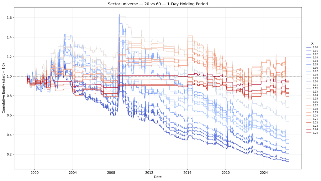
The chart shows a clear distinction between low and high threshold values.
When X is close to 1.00, relatively small increases in short-term correlation are enough to trigger a hedge. The strategy therefore spends considerably more time short SPY. Because the US equity market has a positive long-term drift, frequent short exposure is costly. The lower-threshold variants consequently deteriorate substantially over the full sample. As X increases, the hedge becomes progressively more selective. A stronger increase in cross-sector synchronization is required before a position is opened, the strategy spends less time short SPY, and the equity curves move closer to their initial value.
The important result is not one exact threshold. Instead, a broader region begins to emerge from approximately X = 1.12 to X = 1.25.
The relationship is not perfectly monotonic and individual thresholds still differ. Nevertheless, the higher-X configurations behave materially differently from the low-X part of the parameter grid. This is useful from a robustness perspective. A signal that appeared attractive only at one extremely precise threshold would be much less convincing than a wider region in which the behavior remains economically similar.
The standalone strategy therefore suggests that relatively small increases in market correlation contain limited defensive information. The signal becomes more selective only when short-term correlations move substantially above their medium-term baseline.
However, the standalone short strategy is mainly a diagnostic tool. The more relevant question is whether the same signal improves the behavior of the long equity portfolio it is intended to protect.
We therefore combine the same correlation strategy with SPY Buy & Hold. The combined daily return is calculated as:
combined_return = SPY_return + strategy_return
When no hedge is active, strategy_return equals zero and the portfolio behaves exactly like SPY. When the hedge becomes active, the -1 SPY strategy position offsets the underlying +1 SPY exposure for one trading day. The strategy therefore acts as a temporary risk overlay rather than as a permanent directional short position.
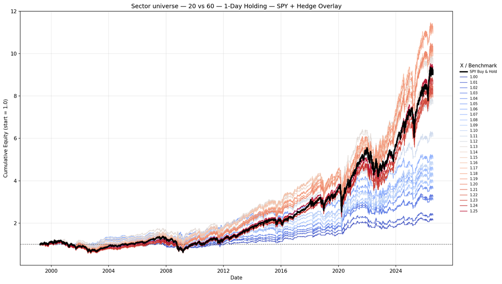
The black curve represents pure SPY Buy & Hold. The colored curves represent SPY combined with the correlation hedge for each X value from 1.00 to 1.25.
The overlay view changes the interpretation substantially. Low threshold values strongly reduce market exposure because the hedge is triggered too frequently. This reduces volatility and drawdowns, but it also removes a large part of SPY’s long-term upside. As X increases, the hedge becomes progressively more selective. The combined portfolio retains more of the underlying equity return while still reducing exposure after stronger correlation shocks.
The complete Sector 20 vs. 60 one-day results are shown below.
| X | Performance | Max Drawdown | Volatility | Sharpe | Calmar |
|---|---|---|---|---|---|
| SPY | 823.00% | -55.08% | 18.94% | 0.52 | 0.15 |
| 1.00 | 118.30% | -30.53% | 11.23% | 0.31 | 0.09 |
| 1.01 | 142.44% | -35.95% | 11.93% | 0.33 | 0.09 |
| 1.02 | 230.41% | -35.17% | 12.56% | 0.41 | 0.13 |
| 1.03 | 216.68% | -36.30% | 13.14% | 0.39 | 0.12 |
| 1.04 | 270.84% | -30.28% | 13.51% | 0.42 | 0.16 |
| 1.05 | 331.55% | -27.96% | 14.53% | 0.44 | 0.20 |
| 1.06 | 416.85% | -30.88% | 14.95% | 0.48 | 0.20 |
| 1.07 | 360.63% | -38.61% | 15.37% | 0.44 | 0.15 |
| 1.08 | 300.75% | -42.06% | 15.63% | 0.40 | 0.12 |
| 1.09 | 334.05% | -43.40% | 15.93% | 0.42 | 0.13 |
| 1.10 | 385.94% | -49.76% | 16.31% | 0.44 | 0.12 |
| 1.11 | 523.92% | -38.87% | 16.60% | 0.49 | 0.18 |
| 1.12 | 681.36% | -39.05% | 16.72% | 0.53 | 0.20 |
| 1.13 | 879.38% | -37.71% | 16.84% | 0.58 | 0.23 |
| 1.14 | 783.77% | -39.78% | 17.02% | 0.55 | 0.21 |
| 1.15 | 923.97% | -39.44% | 17.17% | 0.58 | 0.23 |
| 1.16 | 916.88% | -39.69% | 17.30% | 0.58 | 0.22 |
| 1.17 | 1022.48% | -40.92% | 17.41% | 0.60 | 0.23 |
| 1.18 | 912.44% | -44.25% | 17.60% | 0.57 | 0.20 |
| 1.19 | 1030.36% | -43.43% | 17.65% | 0.59 | 0.21 |
| 1.20 | 935.86% | -44.25% | 17.73% | 0.57 | 0.20 |
| 1.21 | 713.37% | -49.00% | 17.90% | 0.52 | 0.16 |
| 1.22 | 747.17% | -51.64% | 17.99% | 0.52 | 0.16 |
| 1.23 | 729.66% | -49.68% | 18.07% | 0.52 | 0.16 |
| 1.24 | 776.16% | -49.68% | 18.13% | 0.53 | 0.17 |
| 1.25 | 840.78% | -48.11% | 18.18% | 0.54 | 0.18 |
The Sharpe and Calmar values shown in bold correspond to the X = 1.12–1.25 region identified in the robustness review.
The lower part of the parameter grid illustrates the cost of hedging too frequently. At X = 1.00, cumulative performance reaches only 118.30%, compared with 823.00% for SPY. The portfolio experiences substantially lower volatility and a smaller maximum drawdown, but most of the long-term equity return is sacrificed.
The picture changes materially once the threshold reaches the higher-X region. At X = 1.12, cumulative performance remains below SPY at 681.36%, but maximum drawdown improves from -55.08% to -39.05%. Volatility declines from 18.94% to 16.72%, while the Sharpe ratio moves slightly above the benchmark from 0.52 to 0.53. The Calmar ratio increases from 0.15 to 0.20.
At X = 1.13, the combined portfolio already exceeds SPY on cumulative performance, reaching 879.38%. Maximum drawdown is -37.71%, volatility is 16.84%, Sharpe rises to 0.58, and Calmar to 0.23.
Several neighboring parameters continue to produce attractive results. At X = 1.15, cumulative performance reaches 923.97%, with a Sharpe ratio of 0.58 and a Calmar ratio of 0.23. At X = 1.17, cumulative performance reaches 1022.48%, while the Sharpe ratio rises to 0.60. At X = 1.19, cumulative performance reaches 1030.36%, compared with 823.00% for SPY. Maximum drawdown remains lower at -43.43%, while annualized volatility is 17.65%. Even at X = 1.25, cumulative performance reaches 840.78%, slightly above the SPY benchmark, while both volatility and maximum drawdown remain lower.
The main observation is therefore not that one particular X represents the optimal value. The broader X = 1.12–1.25 region contains multiple neighboring configurations with competitive or superior risk-adjusted performance. Several thresholds also outperform SPY on cumulative return.
This broader parameter behavior is more informative than selecting the single strongest historical result.
Rising correlation does not automatically imply a falling market. Equity sectors can become more synchronized during strong rallies, recoveries, major macroeconomic announcements, or other periods when most assets react to the same information.
A threshold close to X = 1.00 therefore reacts to many correlation increases that do not necessarily represent useful defensive signals. This helps explain the weak behavior of the low-X configurations.
Higher thresholds impose a stronger requirement. The strategy no longer reacts simply because short-term correlation moves slightly above its medium-term baseline. Instead, it waits until synchronization has increased by a materially larger amount. The wider high-threshold region suggests that these stronger changes contain more useful information for defensive positioning.
Correlation acceleration should therefore not be interpreted as a direct forecast that SPY will decline on the following day. It is better understood as a measure of how strongly the market is shifting toward common-factor behavior.
The two charts illustrate why the intended role of a quantitative signal matters. The standalone chart asks whether repeatedly shorting SPY after correlation acceleration should be treated as an independent return-generating strategy. The overlay chart asks whether exactly the same signal can improve the behavior of a portfolio that already owns SPY. The second question is more relevant for a hedge.
A defensive overlay does not necessarily need to produce attractive standalone returns. Its role is to alter the risk-return characteristics of the underlying portfolio during periods when protection may be useful. In the Sector 20 vs. 60 experiment, the standalone strategy primarily helps us understand how the threshold controls signal selectivity.
Once the same strategy is combined with SPY, its portfolio value becomes much clearer. Several configurations in the higher-X region produce higher Sharpe and Calmar ratios than SPY. Some also generate higher cumulative performance while maintaining lower volatility and smaller drawdowns than the benchmark.
The main takeaway is therefore not that one exact X value should be treated as the optimal trading parameter. Instead, the results suggest that sufficiently strong increases in cross-sector correlation may provide useful information for selectively timing defensive equity exposure. This is consistent with the broader motivation behind earlier Quantpedia research: correlation information can be useful as a filter that determines when defensive exposure should become active, rather than as a reason to maintain permanent short exposure.
Author: David Mesicek, Junior Quant Analyst, Quantpedia
Are you looking for more strategies to read about? Sign up for our newsletter or visit our Blog or Screener.
Do you want to learn more about Quantpedia Premium service? Check how Quantpedia works, our mission and Premium pricing offer.
Do you want to learn more about Quantpedia Pro service? Check its description, watch videos, review reporting capabilities and visit our pricing offer.
Do you want algorithmic access to the full Quantpedia database via the API? Subscribe to Quantpedia Pro, ask for an API key, and explore the in/out-of-sample statistics, source academic papers, and code snippets — ideal for quantitative research, systematic trading workflows, and AI model training.
Are you looking for historical data or backtesting platforms? Check our list of Algo Trading Discounts.
Or follow us on:
Facebook Group, Facebook Page, Telegram, Twitter, Linkedin, Medium or Youtube
Share onLinkedInTwitterFacebookRefer to a friend