Does More History Help? A Market-Regime HMM and the Trouble with Out-of-Sample Evaluation
This paper investigates whether longer historical training periods improve the out-of-sample performance of a Hidden Markov Model (HMM) used for identifying financial market regimes. Four four-state Gaussian HMMs are compared, differing only in the starting point of their training data (1970, 1980, 1990, and 2000), while being evaluated on the same test period. The model uses five market-based features capturing volatility, drawdowns, credit conditions, and sector rotation to identify latent risk regimes.
The results show that selecting models solely by out-of-sample likelihood can lead to misleading conclusions, favoring shorter training histories that fail to capture crisis regimes. When evaluated using regime stability, economic interpretability, and strategy-based metrics, the model trained on the longest history provides better generalization and avoids overfitting.
The study highlights that validation methodology and evaluation criteria are as important as model design and data length when assessing regime-based investment models.
Introduction
Markets tends to alternate between calm, risk-on conditions — low volatility, tight credit spreads, rising equities — and shorter risk-off episodes in which those conditions reverse. Labelling the prevailing regime is central to much of tactical asset allocation, and this paper studies one approach to it: a Hidden Markov Model (HMM) fit to weekly, market-priced features across six decades. The question we asks is deceptively simple: does training on more history improve out-of-sample generalization? More data is usually better, but financial series are non-stationary, and distant history may contribute noise from a market structure that no longer holds. The choice of training-window start — 1970, 1980, 1990, or 2000, is therefore a bet on how stationary the regime structure actually is.
There is reason to expect it might be. Prices trend without bound, but the features that separate regimes — the level of volatility, its term structure, credit-spread width, drawdown depth — are bounded and mean-reverting; a 40% drawdown in 1974 is the same object as one in 2008. If that structure is stationary, more history should help; if it is not, it should hurt. The experiment is designed to distinguish the two. As the later sections show, however, the harder problem is not asking the question but evaluating it: the validation window and the selection metric determine the answer, and that — more than the model itself — is the contribution of this work.
Background
Hidden Markov Models
An HMM describes a system that occupies one of a small number of hidden states, transitions between them over time, and emits an observable signal whose distribution depends on the current state. The states are never observed directly; they are inferred from the emissions. Two components define the model. A transition matrix gives the probability of moving between states each period and encodes the Markov property — the next state depends only on the current one. A per-state emission distribution — here a multivariate Gaussian over the feature vector — describes what each state tends to produce, so a regime is a distribution of typical volatility, spread, and drawdown values with its own mean and covariance. Parameters are estimated by the Baum–Welch algorithm. The fitted model is then decoded to label each period, and the choice of decoder is consequential: the smoothed estimate uses the full sequence, past and future, whereas the filtered estimate uses only data available up to each point. Any performance evaluation must use the filtered estimate, since the smoothed one incorporates future information and inflates results that could not have been traded in real time.
Why an HMM for market regimes
The model’s assumptions align closely with the problem. Regimes are latent — observable only through their symptoms — persistent, and discrete rather than continuous, which are precisely the properties an HMM encodes through a small state space, sticky transitions, and distinct emission profiles. Relative to simpler alternatives such as a single-indicator threshold or a rolling volatility estimate, an HMM is multivariate, probabilistic, and self-calibrating: it combines several features, returns a regime probability rather than a hard label, and learns its parameters from data. These advantages hold only if the regimes are stable enough to be estimated reliably — which returns to the central question.
Data and features
The feature set is governed by three requirements, each tied to the experiment’s purpose. Features must be stationary, so that a regime can be represented as a fixed Gaussian cloud whose mean and covariance do not drift across the sample; a feature that trended would violate the emission model and confound any comparison across decades. They must have long history, extendable to the early 1960s, since the history-length question cannot otherwise be posed. And they must be market-priced — derived from traded prices and yields rather than surveys or macroeconomic releases — so that they are available in real time, subject to minimal revision, and reflect the market’s own assessment of risk rather than a backward-looking statistic. All inputs come from two free sources: the Kenneth French Data Library (the daily market factor and 12-industry portfolios) and FRED (corporate-bond yields).
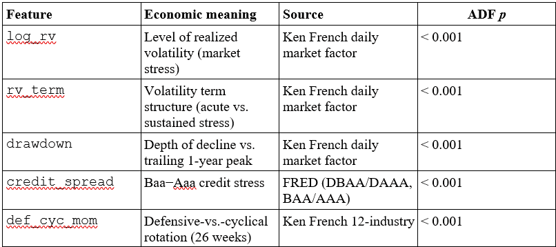
Five features result, spanning four economically distinct channels of risk. Three are computed from the daily total-market return and the price index it implies. log_rv, the log of 21-day realized volatility, captures the level of market stress; it is the single most informative regime signal and the most strongly mean-reverting. rv_term, the log ratio of 21-day to 63-day realized volatility, captures the term structure of volatility — a short-horizon spike relative to the longer horizon marks acute, fast-moving stress, and serves as a model-free substitute for the slope of the implied-volatility curve. drawdown, the price relative to its trailing one-year peak, captures the depth of an ongoing decline and is bounded above at zero by construction.
The remaining two reach beyond the index. credit_spread, the Baa-minus-Aaa corporate yield difference, captures stress transmitted through credit markets, which often widens independently of equity volatility. def_cyc_mom captures cross-sectional rotation: the trailing 26-week relative return of a defensive industry basket against a cyclical one, which turns positive as investors move toward safety. Together the five describe risk as priced in volatility, in its term structure, in price level, in credit, and in sector leadership.
Several construction choices matter for credibility. All features are sampled weekly, on Fridays, and every rolling window is strictly trailing, so no observation incorporates future information. The credit spread is spliced: the daily Baa−Aaa series begins only in 1986, so the earlier period uses the monthly series carried forward onto the weekly grid, with the daily series taking precedence once available. The defensive and cyclical baskets are a deliberate judgment call — defensive as consumer non-durables, healthcare, and utilities; cyclical as durables, manufacturing, business equipment, retail, and finance — with energy, “other,” and a few ambiguous groups left unclassified rather than forced onto one side. The full weekly panel runs from 1962 to the present.
Table 1 summarizes the panel and confirms the stationarity requirement: an augmented Dickey–Fuller test rejects the unit-root null at conventional levels for all five features, with the credit spread the most persistent — unsurprising for a slow-moving credit cycle, and a point we return to when discussing the model’s transition dynamics.
Experiment design
A single chronological split is fixed for the entire study: a training pool covering 1962 through 2009, a test window covering 2010 through 2023, and a sealed holdout from 2024 onward. Against this common backbone, four candidate models are fit, differing only in where their training window begins — 1970, 1980, 1990, or 2000 — each running forward to the same 2010 boundary. Because every variant is then evaluated on the identical test window, the amount of history is the only quantity that varies between them, and the relationship between training-start year and out-of-sample performance becomes a clean answer to the question posed in introduction.
The split boundaries are themselves a deliberate choice, and one that proves consequential. The test window is positioned to contain genuine stress — the 2020 pandemic crash and the 2022 bear market both fall inside it — so that out-of-sample performance reflects a model’s behavior in crisis, not merely its fit to a quiet expansion. The holdout is the recent, low-volatility period from 2024 on, withheld entirely from fitting and selection and reserved for a single final evaluation. As evaluation shows, the decision of where to place the test boundary turns out to matter as much as the history length it is meant to isolate.
The model in each case is a four-state Gaussian HMM with full covariance. The state count is guided by the Bayesian Information Criterion and by interpretability: four states resolve cleanly into a calm regime, a normal regime, a correction, and a crisis, whereas additional states tend to split the calm regime into near-duplicates without adding economic meaning. Full rather than diagonal covariance is necessary because the features are correlated — volatility moves with drawdown, and with credit spreads — and a diagonal model would misrepresent the shape of each regime’s emission cloud. Parameters are estimated by Baum–Welch algorithm with multiple random restarts, since the likelihood is non-convex and a single fit can settle on a poor local optimum.
The discipline around evaluation is what separates this from a backtest that flatters itself, and it is applied uniformly. Standardization is fit on each variant’s training window alone and then frozen; the test and holdout are transformed with those fixed statistics, never their own. The HMM parameters are likewise frozen after fitting and never re-estimated on evaluation data. The holdout is sealed — it informs neither fitting nor selection and is decoded only once, at the very end. All performance evaluation uses the filtered regime estimate, conditioned only on data up to each point, so that no signal can borrow from the future. One further subtlety arises because each variant carries its own standardization: a likelihood computed in standardized space is not comparable across variants, so test likelihoods are reported in raw feature space, correcting for the scaler’s Jacobian, to keep the comparison fair.
How a variant is scored on the test window is, finally, a modelling decision rather than a mechanical one. A model can be ranked by its statistical fit — the test-set likelihood — or by a criterion aligned with its intended use, such as the downside-risk-adjusted return of the regimes it implies. The two need not agree, and here they do not. We defer that choice, and its consequences, to evaluation.
Fitting and the regimes it finds
With the design fixed, each variant is estimated and its regimes decoded across the full sample. Figure 1 presents all four training windows at once: the market price on a log scale, shaded by the regime assigned to each week, with the test window marked.
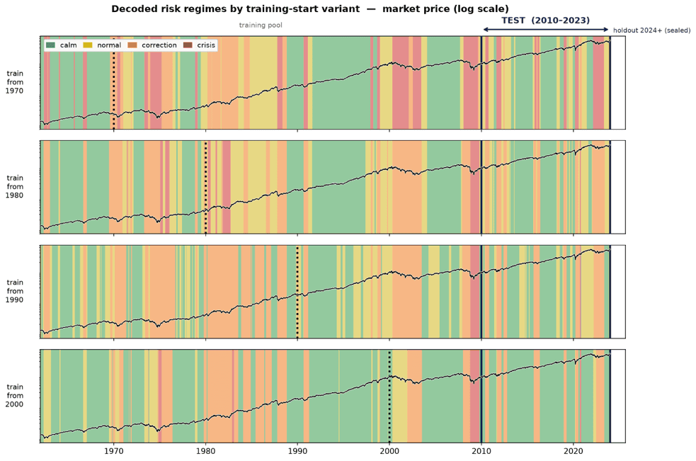
Several features of the figure carry the substance of the experiment. First, the regimes are economically legible: the crisis state coincides with every major historical episode — 1973–74, 1987, 2000–02, 2008, 2020, 2022 — and the correction and crisis states cluster around the visible drawdowns in the price line, while calm and normal dominate the long expansions. Second, and central to the main question, the four panels are broadly consistent but not identical: where a training window begins changes how the early decades are segmented, because a model that never trained on the 1970s is, in those years, extrapolating. The variant beginning in 1970 — which has seen the full range of regimes — labels the early crises most confidently, whereas the later-starting variants decode that period out of distribution. This is the history-length effect made visual.
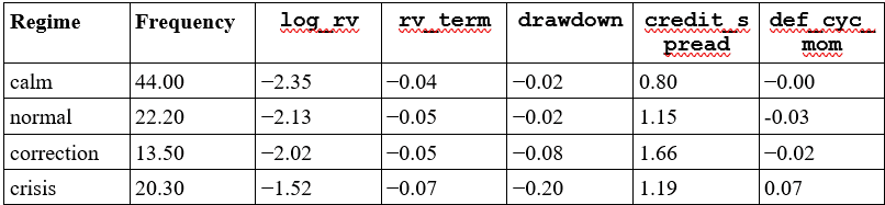
Table 2 gives the regimes their economic identity. Read across the feature means, the four states form not a simple volatility ladder but four distinct risk signatures. Calm and normal are both low-volatility states, separated mainly by credit spreads and sector rotation rather than by volatility itself. The correction state is a credit-stress regime — the widest spreads in the panel alongside only moderate equity volatility — and captures episodes such as the high-spread early 1980s. The crisis state is the equity-volatility regime, marked by the highest realized volatility and the deepest drawdowns, and it is where 1987, 2008, and 2020 fall. That the most informative split is between credit stress and equity stress, rather than along a single intensity axis, is itself a useful output of the model.
Does more history help?
The four variants are compared on the common test window; Table 3 reports the sweep. Ranked by out-of-sample likelihood — the obvious scalar — the recommendation is one of the shorter-history models, the variant beginning in 1990. Taken at face value, this answers the title question in the negative: more history does not help.
Two parameters contradict that reading. The first is the number of regimes each model expresses out of sample. Practically only the variant trained from 1970 uses all four states on the test set; The shorter shorter-history models used crisis state only marginally or collapsed to three, leaving the crisis state empty. For a model whose purpose is to flag crises, an unpopulated crisis state is not a minor defect but the failure mode itself. The second is the gap between in-sample and out-of-sample likelihood. Smallest values for the 1970 and 1980 variant, widens steadily as the training window shortens. That is the signature of overfitting. The short-history models fit their recent, quiet training data tightly and fail to carry the fit forward.
The reason the scalar misleads is structural. Out-of-sample likelihood is an average over the test window, and any plausible window is composed overwhelmingly of calm weeks; even after the window is deliberately positioned to include the 2020 and 2022 selloffs, those episodes remain a small minority of observations. A model is therefore rewarded for fitting the placid majority and barely penalized for mislabeling the few weeks that matter. The correction has two parts. Placing genuine stress inside the validation window gives crisis detection at least some weight; more decisively, ranking the variants by a criterion aligned with the model’s use — the downside-risk-adjusted return of the regime-driven strategy each implies — rather than by raw fit reverses the ordering. Under that criterion the longest-history model, alone in having trained across the full range of historical regimes, generalizes best.
The answer to the title question is therefore yes — more history does help. It lets the model populate a crisis state and resist overfitting a calm recent window. Yet that conclusion is invisible to the metric most naturally reached for, and a practitioner who selected on out-of-sample likelihood over a quiet decade would have shipped the overfit, crisis-blind model and concluded, wrongly, that the past is noise. The history-length question cannot be separated from the evaluation that surrounds it. The validation period and the scoring metric determine the answer at least as much as the training length ostensibly under study.
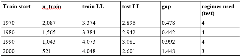
Per-observation log-likelihood, raw feature space; gap = train − test, with larger values indicating more overfitting. Likelihood alone ranks 1990 first.
Does it work?
Whether the regimes are worth trading is a separate question from whether they are real, and it is an easy one to answer dishonestly. A model that cuts equity exposure in its correction and crisis states will mechanically carry less risk than a fully invested benchmark, and in a sample containing large drawdowns it will usually post a higher Sharpe ratio for that reason alone. The relevant question is not whether the strategy beats buy-and-hold, but whether it beats its own de-risked shadow — a portfolio holding the same average exposure on a fixed schedule, with no regime information at all. If it cannot, its apparent skill is beta reduction in disguise.
Table 4 makes that comparison directly, setting the regime strategy beside two information-free twins — a static portfolio matched to its average exposure, and a volatility-targeted portfolio that scales exposure by inverse realized volatility — and against a permutation test that reshuffles the regime blocks while preserving their length. The result is a modest one. The strategy’s edge over its static twin is slightly negative, its Sharpe does not exceed the volatility-targeted twin, and the permutation test fails to reject: the actual Sharpe sits below the average of the strategy’s own reshuffled histories. The HMM does reduce maximum drawdown — it genuinely holds less through crises — but there is no evidence of timing skill beyond what a naive volatility rule already captures. It de-risks; it does not time. A regime classifier can be genuine, as these regimes plainly are, and still deliver no tradable edge.
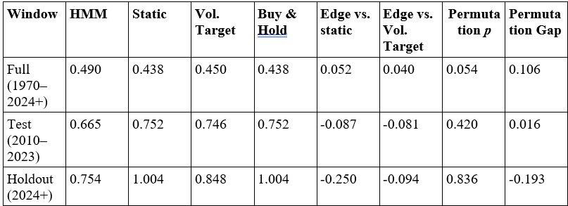
The static twin holds the strategy’s average exposure on a fixed schedule; its Sharpe equals buy-and-hold’s by construction, making it the yardstick the HMM must clear. “Edge vs. static” isolates timing from de-risking.
Conclusion
The experiment asked whether a market-regime model benefits from more training history, and the answer is a qualified yes. More history helps: the longest-history variant is the only one to represent all four regimes out of sample, and the only one to avoid overfitting a calm recent window. But that benefit is real only when the evaluation is capable of seeing it.
The more durable finding is methodological. A single natural scalar gave a confident, wrong answer, and the honest answer emerged only from a use-aligned criterion. Out-of-sample likelihood recommended the overfit, crisis-blind model; the evaluation of populated regimes and the train–test gap corrected it. The decisive choice was the yardstick, not the model. For regime modeling in particular, this means that the choice of validation period and selection metric can have same value as the training length, the state count, or the feature set — the parameters that usually absorb the most attention.
As for the model, it is a competent classifier and an unremarkable strategy: its regimes align with history and carry economic meaning, but it de-risks rather than times and does not beat a simple volatility rule. A model that is clearly finding something real yet delivers no tradable edge is not a failure of the exercise but its most instructive outcome, visible only because the evaluation was built to reveal it rather than to flatter it.
Author: Julián Jalšovský, Quant Analyst, Quantpedia
Are you looking for more strategies to read about? Sign up for our newsletter or visit our Blog or Screener.
Do you want to learn more about Quantpedia Premium service? Check how Quantpedia works, our mission and Premium pricing offer.
Do you want to learn more about Quantpedia Pro service? Check its description, watch videos, review reporting capabilities and visit our pricing offer.
Do you want algorithmic access to the full Quantpedia database via the API? Subscribe to Quantpedia Pro, ask for an API key, and explore the in/out-of-sample statistics, source academic papers, and code snippets — ideal for quantitative research, systematic trading workflows, and AI model training.
Are you looking for historical data or backtesting platforms? Check our list of Algo Trading Discounts.
Or follow us on:
Facebook Group, Facebook Page, Telegram, Twitter, Linkedin, Medium or Youtube
Share onLinkedInTwitterFacebookRefer to a friend