Introduction and Examples of Monte Carlo Strategy Simulation
The Monte Carlo method (Monte Carlo simulations) is a class of algorithms that rely on a repeated random sampling to obtain various scenario results. Monte Carlo simulations are used to predict the probability of different outcomes when it would be difficult to use other approaches such as optimization. The main aim is to create alternative scenarios, which account for possible risk and help with decision making. The simulations are used in various fields, from finance and quantitative analysis to engineering or science. We plan to unveil our new “Monte Carlo” report for Quantpedia Pro clients in a next few days, and this article is our introduction to different methodologies that can be used for Monte Carlo calculation.
Monte Carlo Simulations are a useful tool both for risk management and portfolio management. Risk managers may calculate a proper budget for a potential quantitative investment strategy, whereas portfolio managers may set their expectations more precisely and easily perform a sensitivity analysis of their strategies. Monte Carlo simulations are an option to create endless alternative scenarios to test your strategies in. Their main advantage is that they reach beyond historical data and rather alter the history artificially.
Underlying Strategy
In our analysis, we applied Monte Carlo simulations to a quantitative investment strategy. More specifically we used a trading strategy called a Return Asymmetry Investment factor in commodity futures. The strategy is based on the idea that the greater (lower) upside asymmetry is associated with lower (higher) expected returns, analyzed in numerous theoretical studies.
Quantpedia’s commodity futures strategy aims to examine the return asymmetry in commodity futures in a slightly less traditional way. Instead of using skewness as a proxy for the return asymmetry, we rely on a new asymmetric measure IE proposed by Jiang et al. (2020), which uses the difference between upside and downside return probabilities to capture the degree of asymmetry.
As for the investment universe, the strategy follows Padyšák and Vojtko (2019). Their dataset of commodities offers broad exposure to the commodity market. The portfolio is constructed on the asymmetric measure as follows. At the beginning of each month, each commodity’s asymmetry (IE) is calculated using the latest 260 daily returns. Then the commodities are ranked according to their IE. The portfolio goes long on the bottom four commodities with the lowest IE in the previous month and short on the top four commodities with the highest IE in the last month (ties in ranks can change these).
Monte Carlo strategy simulation types
There are several types of Monte Carlo applications in quantitative trading strategies. We will focus on different ways of randomization of strategy’s returns. In this article we cover the most practical and most widely used ones:
- Monte Carlo sampling without replacement
- Monte Carlo sampling with replacement
- Monte Carlo return alterations
- Comparison against random strategies
Now, we can (and we do) apply each of these to either:
- Period returns of the strategy (e.g. monthly returns) or
- Trade returns of the strategy
With period returns it’s more of a time series approach, while with trade returns it’s more a classical trading P&L point of view.
Analysis
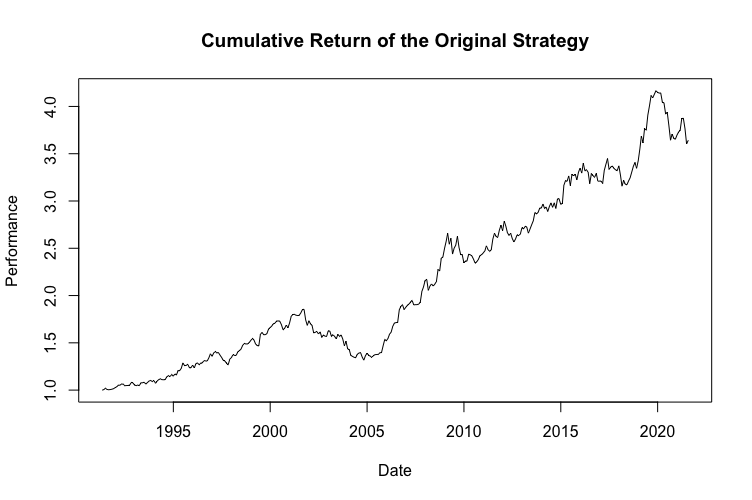
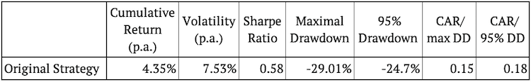
As we already mentioned, we applied Monte Carlo simulations to an already existing strategy. The following figure shows the cumulative performance of the original, unaltered strategy and also its risk and return characteristics.
Our analysis consists of three parts, each including multiple approaches to Monte Carlo simulations:
- The first part analyzes the monthly returns of the strategy and applies the first three Monte Carlo methods mentioned above
- The second part does the same, but utilizing trade returns
- Finally, the third part presents the comparison of the original strategy against random strategies
Monte Carlo simulations of the Strategy’s Monthly Returns
In the first section, we look at the monthly returns of the underlying strategy. First of all, we create a vector of monthly returns. Then we take three approaches to Monte Carlo simulations to create new vectors.
Monte Carlo sampling without replacement
This Monte Carlo method only changes order of the returns, i.e. “reshuffles” returns. The main assumption behind this method is, that returns will stay the same (or similar) but their order of occurrence may change.
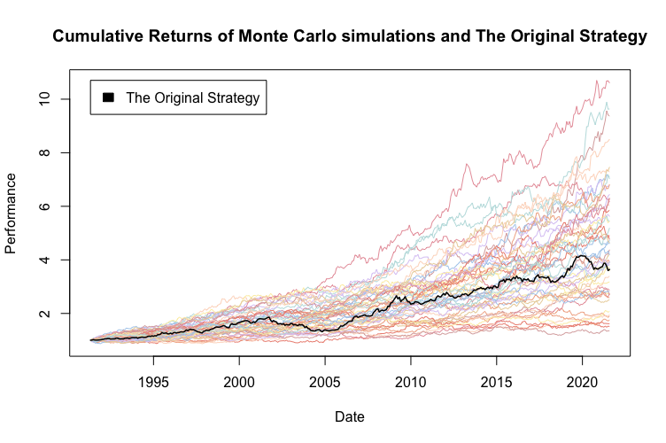
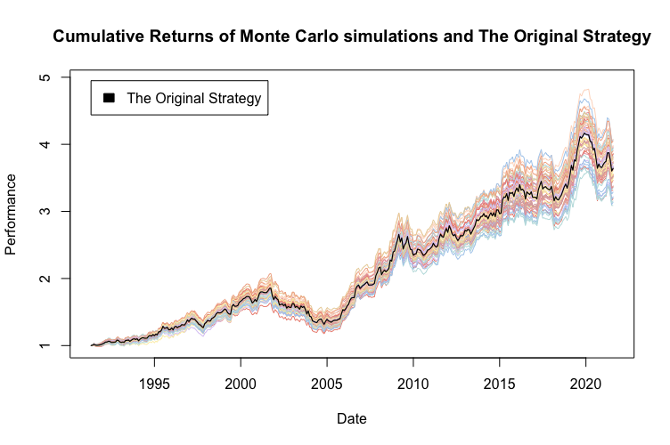
Technically we are talking about a simple random sampling without replacement (reshuffling the data). We create 100 new samples of the same length by applying randomization without replacement. So, we basically reshuffle the data 100-times to create 100 new vectors, and we calculate the cumulative returns of the simulated strategies. For better visual clarity, the following figure shows only 50 of the 100 simulations.
When using Monte Carlo random sampling without replacement, the volatility of the simulated strategies will be always the same as that of the original strategy. Also, the cumulative return will be logically very similar, because we only change order of the returns and the only way why return may differ is because of compounding. The most interesting attribute to observe in this Monte Carlo method is drawdown. Drawdown may change (and also does change in our case) significantly when we change the order of the returns.
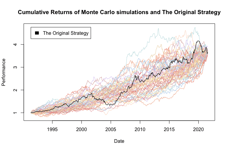
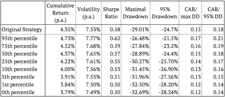
The figure above presents various random realizations of return order reshuffling. The figure also shows that the original strategy lies roughly in the middle of the simulated strategies most of the time, exactly as expected. We calculated the 95th, 75th, 50th, 25th, 10th, 5th, 1st, and the 0th percentile of the risk and return characteristic to see exactly how well it performs compared to the simulations.
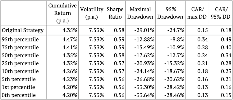
Interestingly enough, more than 95% of the random realizations have lower (better) drawdown figure than the original strategy. This suggests, the original’s strategy drawdown may be a bit conservative figure.
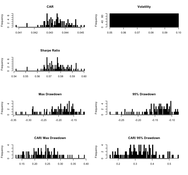
Additionally, the next figure presents a set of histograms showing the frequency of individual risk and return characteristics in our 100 simulations. There is only a single value for volatility because we applied the random sampling without replacement.
Monte Carlo sampling with replacement
This Monte Carlo method not only changes order of the returns, it also randomly skips or repeats returns of the original strategy. The main assumption behind this method is, that a return distribution will stay the same (or similar) but returns may change more significantly.
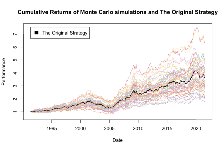
Technically, we are talking about a random sampling with replacement. We create 100 new samples of the same length as the original vector of returns by applying randomization of returns with replacement. Then we calculate the cumulative returns of the simulated strategies. For better clarity, the figure below again shows only 50 of the 100 simulations.
Monte Carlo sampling with replacement creates much more variety in simulated strategy returns. It’s logical that randomization with replacement may result in repeating multiple unsuccessful months as well as multiple successful ones in a row. With this method we also simulate changes in volatility and in cumulative returns.
Once again, as expected, most of the time the original strategy seems to lie in the middle of the simulated strategies. Again, we calculated the 95th, 75th, 50th, 25th, 10th, 5th, 1st, and the 0th percentile of the risk and return characteristic to see how well the original strategy performed.

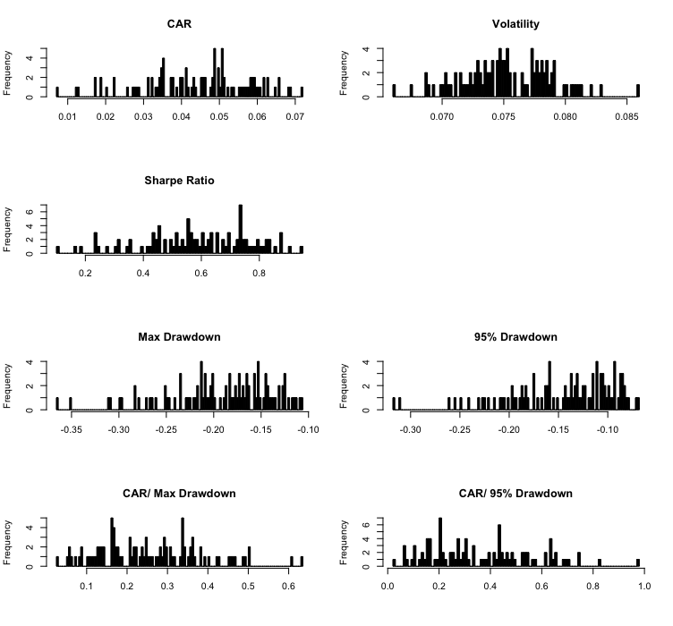
Looking at the cumulative return, volatility, and Sharpe ratio, the original strategy’s performance is between the 25th and the 50th percentile. This indicates, that more than half of the random alterations of the strategy are eventually better than the original strategy. When we look at the maximum drawdown or the 95% drawdown, once again they are better than the original strategy in more than 95% of scenarios. This is definitely encouraging for the original strategy. Moreover, we present a set of histograms showing the frequency of individual risk and return characteristics.
Monte Carlo return alterations
This Monte Carlo method changes randomly picked returns in random direction by a pre-specified amount. The main assumption behind this method is, that returns may simply become smaller or larger in the future. It’s useful to observe strategy’s sensitivity to such a scenario.
Technically, we change X% of the data by Y%. So, in the first step, we randomly choose X% of the returns, and then we randomly either add Y% to or subtract Y% from the chosen monthly return in the second step.
For example, if the monthly returns were (0.5%, 1%, -2.5%, -3%, 0.5%, 1.5%), X = 0.5 (50%) and Y = 0.02 (2%). One of the simulations could be (2.5%, -1%, -2.5%, -5%, 0.5%, 1.5%). The process is repeated 100-times with the same X and Y for all simulations, and cumulative performances are calculated.
We used X = 0.5 (50%) and Y = 0.02 (2%) in all of our simulations. For better clarity, the following figure shows only 50 of the 100 simulations.
Logically, by changing half of the returns, we only increase the volatility of the simulations for the majority of the time. This can also be observed in empirical results. The same applies to drawdown. On the other hand, returns oscillate around the original strategy, as expected.
Once again, the original strategy’s performance is in the middle of the simulated strategies – this time exactly as expected. Next, we calculated various percentiles of the risk and return characteristic to see how well the original strategy performed compared to Monte Carlo simulations.
Lastly, we present a set of histograms that show the frequency of individual values of risk and return characteristics.

Monte Carlo simulations of the Trades
In the second section, we apply all 3 methods analyzed above, however not to simple monthly returns as above, but rather to the results of the individual trades of our strategy. By “a trade” we understand return of a long or a short position for every individual commodity. It’s interesting to observe the differences between looking at strategy’s pooled monthly returns only and looking at individual trades’ returns.
Monte Carlo sampling without replacement
We analyze the same three approaches to Monte Carlo simulations. The first one is a simple random sampling of trades without replacement. For clarity, the following figure shows only 50 of the 100 simulations:
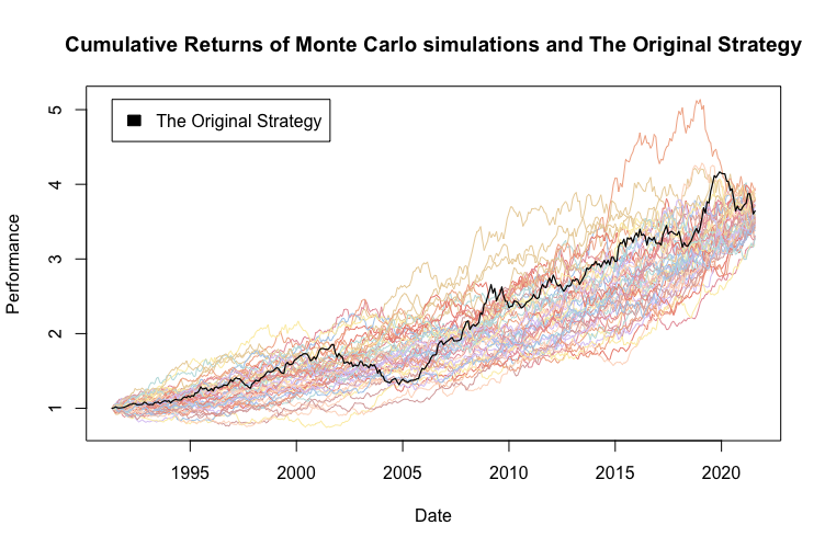
When sampling trades’ returns without replacement, the volatility of the simulated strategies may or may not be the same as that of the original strategy. This depends on the strategy construction. In our case it varies slightly. The same applies to returns generated by these Monte Carlo trades simulations. Drawdown is logically entirely different by definition.
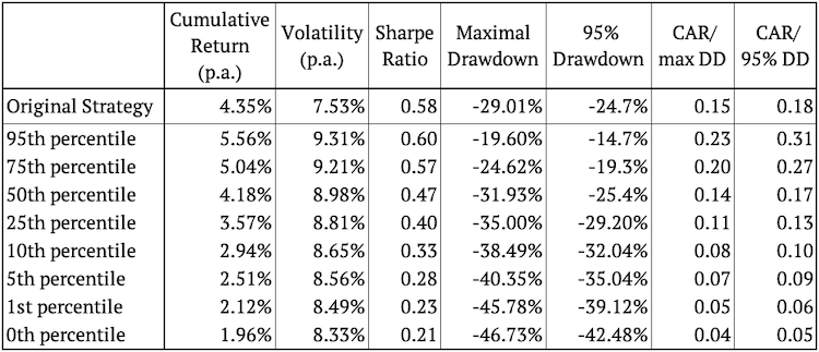
The following table shows the percentiles of risk and return characteristics of the simulations and the risk and return characteristics of the original strategy.

We may observe the same phenomenon as with the monthly returns – in most of the simulations the drawdown figure is better than for the original strategy. Additionally, we also plotted the histograms with the frequencies of values of risk and return characteristics.

Monte Carlo sampling with replacement
Secondly, we sample 100 new matrices by applying sampling with replacement to trades. The monthly returns of each of the 100 new strategies are calculated and the cumulative returns are plotted. For clarity, the following figure shows only 50 of the 100 simulations:
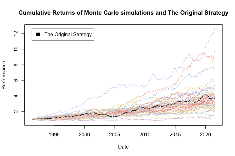
Sampling with replacement always produces higher dispersion in results compared to Monte Carlo sampling without replacement. This is also the case for simulation trade returns. We may observe that the volatility of Monte Carlo simulations is noticeably higher and there are multiple outliers in the simulated returns.
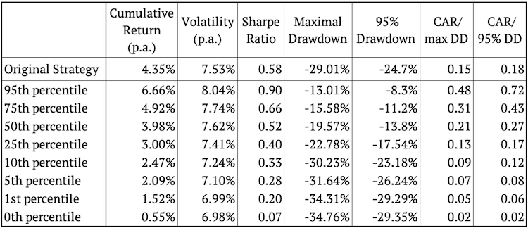
The table shows that the Maximum Drawdown figure still tends to be better for most of the simulations.

Monte Carlo return alterations
The third approach changes X% of the trades by Y%. The process is repeated 100-times with the same X (50%) and Y (2%) for all simulations, and performances of the simulated strategies are calculated. For clarity, the following figure again shows only 50 of the 100 simulations:
In our case, Monte Carlo return alteration doesn’t result in a big variation of simulated equity curves. The reason is our strategy construction (equal weighing trades) which mostly averages out our random return alterations.
This time, the conclusion from this analysis is pretty neutral. The median of Monte Carlo simulations oscillates roughly around the original strategy in all performance metrics. Additionally, we can analyze the following histograms showing the frequencies of values of individual risk and return characteristics.

Comparison against Random Strategies
This Monte Carlo method is utilized to create a set of random strategies to compare the original strategy against. It is based on assumption that your original strategy should outperform majority of the random strategies.
We again use data on individual trades. Technically, we firstly randomly choose which commodities are traded each month. Secondly, we randomly go long, or short, or stay in cash with each chosen commodity. The process is again repeated 100-times. For clarity, the following figure shows only 50 of the 100 simulations:
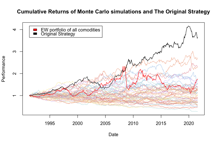
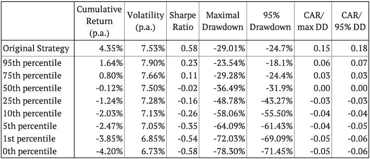
Random trades by definition oscillate around zero for the majority of time. This should be one of the easier hurdles for your strategy to pass. This Monte Carlo testing set serves as an independent (of your strategy) benchmark which should be outperformed.

Comparison of different Monte Carlo methods
We analyzed and presented results for 4 different Monte Carlo simulations methods applied to a commodity futures trading strategy. We applied them to both – monthly returns of the strategy and single individual trades of the strategy.
Monthly returns vs. Individual trades
The choice whether to use time-series returns (e.g. monthly) or trades’ returns highly depends on your needs. If you are a swing trader who focuses on each separate trade then probably the trade analyzes would be more suitable for you. On the other hand, if you are a diversified investor who averages different assets or different approaches then time-series returns (period returns) should be easier for you to use.
Monte Carlo strategy simulations without replacement
One of the softer Monte Carlo simulations for trading strategies is sampling without replacement. This method only changes the order of returns. Hence, it doesn’t change volatility, nor average return. It’s mainly useful for drawdown analysis and for examination of shapes of strategies’ equity curves. It’s the stress test for those, who expect similar returns for the strategy in the future, just occurring at different times.
Monte Carlo strategy simulations with replacement
Monte Carlo sampling with replacement is probably the most widely used method for simulating hypothetical scenarios of quantitative strategies. By using simulations with replacement, we create several “new histories” and randomize also return and risk of the strategy. It’s used by those who believe the returns of the strategy will be distributed roughly similarly in the future, but who don’t believe they will be same.
Monte Carlo return alteration
Monte Carlo alteration of strategy’s returns is basically a sensitivity analysis and should be used and perceived like that. It helps to analyze how big is the impact of pre-specified random changes to a pre-specified share of strategy’s returns. The less deteriorated the simulation results are, the better.
Comparison against random strategies
Probably everybody knows a Malkiel’s monkey beating stock markets. It’s always useful to take a look how your strategy performs against random strategies. And this is exactly the purpose of this Monte Carlo method. Logically, one would expect their strategy to outperform random variants convincingly.
Conclusion
We presented, explained and analyzed multiple approaches to Monte Carlo simulations. We also performed a real case study of Monte Carlo simulations applied to a commodity futures trading strategy.
Different Monte Carlo methods may be valuable for different end-users. It’s crucial to understand how they work and how to interpret them. You can learn that easily from our article above.
Author:
Daniela Hanicova, Quant Analyst, Quantpedia
Are you looking for more strategies to read about? Sign up for our newsletter or visit our Blog or Screener.
Do you want to learn more about Quantpedia Premium service? Check how Quantpedia works, our mission and Premium pricing offer.
Do you want to learn more about Quantpedia Pro service? Check its description, watch videos, review reporting capabilities and visit our pricing offer.
Do you want algorithmic access to the full Quantpedia database via the API? Subscribe to Quantpedia Pro, ask for an API key, and explore the in/out-of-sample statistics, source academic papers, and code snippets — ideal for quantitative research, systematic trading workflows, and AI model training.
Are you looking for historical data or backtesting platforms? Check our list of Algo Trading Discounts.
Or follow us on:
Facebook Group, Facebook Page, Telegram, Twitter, Linkedin, Medium or Youtube
Share onLinkedInTwitterFacebookRefer to a friend


