Introduction to Clustering Methods In Portfolio Management – Part 1
At the beginning of October, we plan to introduce for our Quantpedia Pro clients a new Quantpedia Pro report dedicated to clustering methods in portfolio management.
The theory behind this report is more extensive; therefore, we have decided to split the introduction into our methodology into three parts. We will publish them in the next few weeks before we officially unveil our reporting tool. This first short blog post introduces three clustering methods as well as three methods that select the optimal number of clusters. The second blog will apply all three methods to model ETF portfolios, and the final blog will show how to use portfolio clustering to build multi-asset trading strategies.
Use of Portfolio Clustering
In one of the previous posts, we introduced Risk Parity Asset Allocation. It is an investment management strategy that focuses on risk allocation. The main aim is to find assets’ weights that ensure an equal level of risk, most frequently measured by volatility. However, naive risk parity methods do not take into consideration a type of asset class and the number of assets in each asset class.
Let’s present an example of naive risk parity weighting in two different investment baskets.
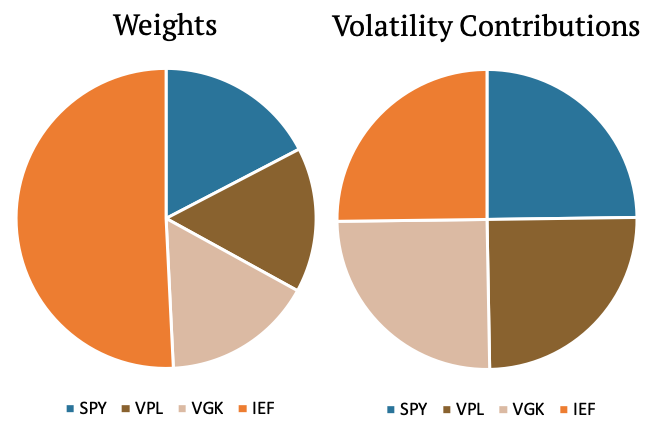
In the first example, we have three equity assets (SPY, VPL, VGK) and one bond (IEF). We apply risk parity methodology (we weight assets inversely to their volatility), and as we can see in the figure below on the right, the volatility contribution of all four assets is equal. The weight of the bond makes up about half of the portfolio; however, its volatility contribution is just one quarter. That’s because there is just one bond ETF but three equity ETFs in the first investment basket.
What if we wanted the volatility contribution of all equity assets together to be equal to the volatility contribution of all fixed-income assets?
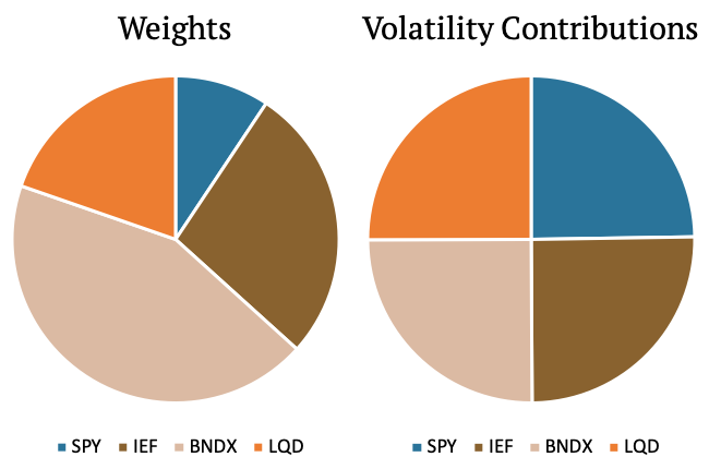
The second example shows a different portfolio. This portfolio is made up of three bond ETFs (IEF, BNDX, LQD) and one equity ETF (SPY). As we can see, the weight of SPY is now much lower compared to the example above, yet it makes up the same 25% of the volatility contribution. The examples above shows that it might be desirable to find such weights that equities together would make up half of the volatility contribution and the bonds together would make up the other half.
| Algo Trading Data Discounts are available exclusively for Quantpedia’s readers. |
What’s the take-away? A naive risk parity method is undesirably sensitive to the number of assets from a particular asset class. Is it possible to overcome this issue? Yes, it is. Firstly, we have to group the assets into categories (equity-like, bond-like, commodity-like, etc.). This can be done either manually or automatically e.g. by the technique called portfolio clustering. And exactly, portfolio clustering will be our focus today. Once we cluster the assets well enough, we can run a traditional risk parity scheme. Risk allocation to each “group” of assets will be then equalized – which is our aim.
Clustering
One of the first things people learn from an early age is to sort things into categories. Humans love to categorize items based on a variety of criteria: size, color, price, material, and so on. It is very natural for us to put things into boxes. And, just like in everyday life, it is very useful to be able to categorize things in the financial world.
Clustering is the act of grouping objects in such a way that the objects in the same group, called a cluster, are more similar to one another than to the objects in the other groups – clusters.
There are numerous ways to cluster an object such as an asset in a portfolio. In this article, we present several methods that deal with clustering, all with an application to trading strategies. We introduce three of the most popular clustering methods – Hierarchical Clustering, Centroid Method (specifically Partitioning Around Medoids), and Gaussian Mixture Models.
Clustering Methods
We will now dive into the clustering itself. In this section, we introduce several clustering methods, and in the later section, we show examples of all of the methods used in portfolio management.
Partitioning Around Medoids
Partitioning Around Medoids (PAM) is a type of centroid based clustering method. These methods are considered one of the most simplistic yet the most effective ways of creating clusters. The idea behind centroid based clustering is that a central vector (called centroid) characterizes a cluster, and data points closest to these vectors are assigned to the respective clusters.
The first step one has to take is to preset a number of clusters and assign random objects to each cluster. Then the centroid can be calculated for each of the clusters. Precisely, for PAM, the centroid is calculated as a medoid (an object whose average dissimilarity to all the objects in the cluster is minimal) of the objects in each cluster. After that, the algorithm creates new clusters based on the proximity to the medoid, and the new medoid is calculated for the newly created clusters. This is repeated until the clusters no longer change.
A major disadvantage of this method is that we have to predetermine the number of clusters. It can be done either intuitively or scientifically using one of the methods we will analyze below.
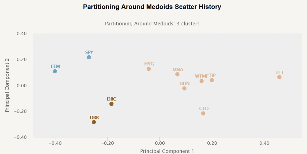
The following figure illustrates data categorized into three clusters using the PAM method.
Partitioning Around Means
Since November 2024, the Portfolio Clustering report has switched to using the Partitioning Around Means algorithm. The key difference in comparison to the previous method is how it represents clusters:
-
Medoids: It uses an actual data point to represent a cluster. It’s the point within the cluster that minimizes the average dissimilarity (or distance) to all other points in the dataset. Because medoids are real data points, they’re more robust to noise and outliers, especially when using distance measures that don’t rely on mean calculations.
-
Means: It uses the arithmetic mean (average) of a cluster’s data points. In other words, it’s a computed central point that doesn’t necessarily have to be an actual data point. It can be sensitive to outliers, as outliers can skew the mean position. However, we don’t observe huge differences from the practical perspective and consider this approach an adequate substitution.
Hierarchical Clustering
Another widely used method of clustering is hierarchical. This method uses machine learning to create a hierarchy of objects to put into clusters. There are two main approaches based on the direction of progress: top-down (Divisive Approach, also known as DIANA) and bottom-up (Agglomerative Approach, also known as AGNES).
The top-down approach starts with one data set that contains all of the objects (1 cluster). Then, the objects are gradually divided into smaller groups, ending in clusters. This approach is best suited for identifying large clusters.
The bottom-up approach starts with each object in its individual group (cluster). Then the groups are gradually being merged, creating bigger groups, which end in clusters. This approach is ideal for identifying smaller clusters.
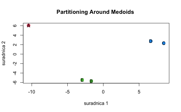
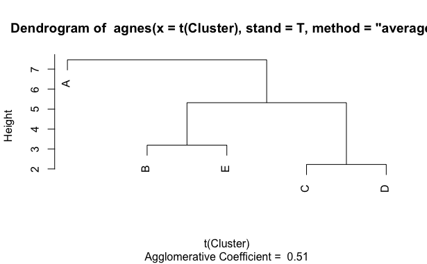
The following figure (the so-called dendrogram) shows the same data categorized using the agglomerative approach. Clusters would be created by cutting the tree at a chosen height. For example, if we chose to cut the tree at the height of 4, we would get three clusters. The first cluster would contain object A, the second would contain B and E, and the last cluster would contain objects C and D. On the other hand, if we e.g. cut the tree at the height of 3, we would get four clusters (first with C+D and then three single object clusters of A, B and E).
That’s nice. But where to cut the tree? We will get into it in the next section.
Gaussian Mixture Model
Both of the clustering techniques above are based on the proximity of the data points. However, there is a class of clustering algorithms that considers a different metric – probability. Distribution-based clustering groups data based on their likelihood of belonging to the same probability distribution. In our case, the assumed distribution is Gaussian.
Gaussian Mixture Model (GMM) assumes that the data points follow Normal (Gaussian) distribution. If they don’t, a normalization of the data is required. This assumption leads to important selection criteria for the shape of the clusters. With Gaussian Mixture Model, we are able to quantify clusters using mean and variance.
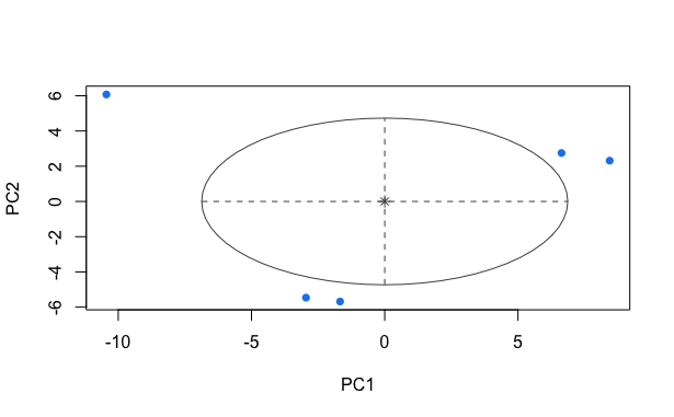
This method chooses the number of clusters by itself. For example, in the figure below, we can see that this method sorted all the data points into one cluster.
Selecting the optimal number of clusters
Now that we know what is clustering and how it categorizes data, we need to address one crucial topic. How to decide on the number of clusters? This is an important step in both PAM and hierarchical clustering described above. There are numerous scientific ways to determine the optimal number of clusters. Let us introduce three commonly used methods.
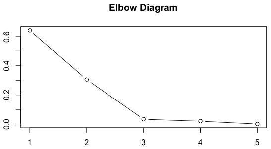
The first one is the Elbow Method. The elbow method is one of the most popular methods for determining the number of clusters. It consists of plotting the explained variation of data points as a function of the number of clusters. The decision rule on the number of clusters is then based on picking the elbow of the curve as the number of clusters to use (i.e. finding a “break” in the elbow diagram). For example, in the figure below, the optimal number of clusters according to this method would be three.
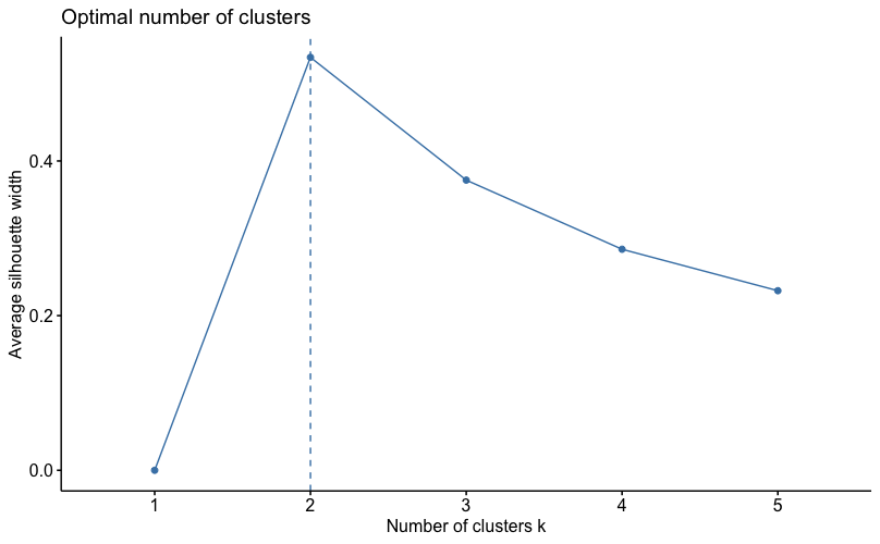
Another widely used method is the Silhouette Method. The silhouette value measures how similar an object is to its own cluster compared to other clusters. It is based on the average distance of an object to the other clusters. The silhouette ranges from 0 to 1, where a high value indicates that the object is well matched to its own cluster and poorly matched to other clusters. If most objects have a high value, the clustering is done well. On the other hand, if many objects have a low silhouette value, the clustering may have too many or too few clusters. The silhouette method thus provides a representation of how well each object has been classified.
As we can see in the figure below, the silhouette method would recommend sorting objects into two clusters.
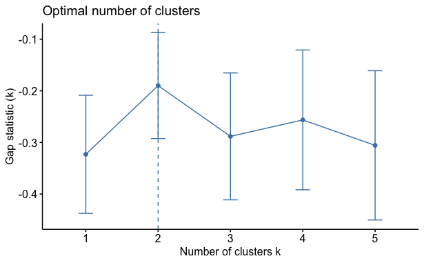
Last but not least, we introduce the Gap Statistic. The Gap Statistic standardizes the log(W) graph, where Wis the within-cluster dispersion, by comparing it to its expectation under an appropriate null reference distribution of the data. Then the estimate of the optimal number of clusters is the value that maximizes the gap statistic. This means that the clustering structure is far away from the random uniform distribution of points.
Based on the results of the Gap Statistic illustrated below, we would sort the data into two clusters.
Conclusion
There are countless clustering methods. In this article, we introduced three of them. If you are asking which of these methods is the best, there is no correct answer. Overall, each method has its pros and cons. The selection of a specific method should depend on the type of data one needs to cluster. Additionally, the method for selecting the number of clusters is equally important. Ultimately, we suggest applying at least two clustering methods and comparing the final results before settling on one final method.
The second blog post from the clustering series analyses the three abovementioned clustering methods on real (investment) life data, including equity, alternative, and bond ETFs.
Author:
Daniela Hanicova, Quant Analyst, Quantpedia
Are you looking for more strategies to read about? Sign up for our newsletter or visit our Blog or Screener.
Do you want to learn more about Quantpedia Premium service? Check how Quantpedia works, our mission and Premium pricing offer.
Do you want to learn more about Quantpedia Pro service? Check its description, watch videos, review reporting capabilities and visit our pricing offer.
Are you looking for historical data or backtesting platforms? Check our list of Algo Trading Discounts.
Would you like free access to our services? Then, open an account with Lightspeed and enjoy one year of Quantpedia Premium at no cost.
Or follow us on:
Facebook Group, Facebook Page, Twitter, Linkedin, Medium or Youtube
Share onLinkedInTwitterFacebookRefer to a friend