Time Invariant Portfolio Protection
INTRODUCTION
In this article we are going to continue the discussion on portfolio insurance strategies. An exhaustive description of this methodology was already presented in the article Introduction to CPPI (https://quantpedia.com/introduction-to-cppi-constant-proportion-portfolio-insurance). This article will focus on an extension of the original model introduced by Estep and. Kritzman (1988), namely Time Invariant Portfolio Protection.
Constant Proportion Portfolio Insurance (CPPI) and Time-Invariant Portfolio Protection (TIPP) are two of the most famous portfolio insurance strategies that play an important role in the realm of investment management and risk mitigation. These strategies are designed to address the fundamental challenge of balancing the pursuit of financial growth with the imperative of capital protection against market downturns. Ideally, the guaranteed protection is achieved at the lowest possible premium for the investors.
THE MODEL
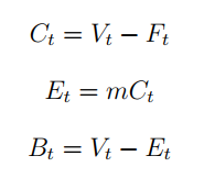
CPPI is a dynamic approach that adapts to market conditions by actively adjusting the allocation between risky and risk-free assets, striving to preserve a predefined floor value while allowing participation in market upswings. In contrast, TIPP employs a more conservative methodology, where a fixed percentage of portfolio value is guaranteed throughout the investment horizon and the risky exposure is adjusted accordingly. The main difference is that while in CPPI the floor grows at a constant rate, in TIPP it is a function of the portfolio value and thus it has a path dependent nature. These two strategies offer distinct advantages and drawbacks, making them valuable tools for investors with varying risk appetites, investment objectives, and preferences for portfolio management.
Both strategies prescribe an allocation to the risky asset that is equal to the cushion (difference between V0 and F0) multiplied by a risk-aversion coefficient m. The higher the coefficient, the more aggressive the strategy, and conversely. The allocation to the risk-free is determined residually.
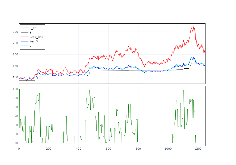
Let’s show an example. If we assume an initial invested capital of 100$, an initial floor of 85$, and a multiplier of 4, we obtain a risky exposure of 60 (4x(100-85)) and risk-free allocation of 40. Many finance practitioners have introduced new extensions to the plain vanilla model. For instance, setting on the maximum and minimum exposure will avoid, on one side, excessive risk taking and on the other hand, the absorption in state of 100% risk-free allocation. In our experiment, we force the exposure to lie in the range 40 to 120%.
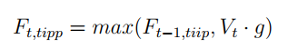
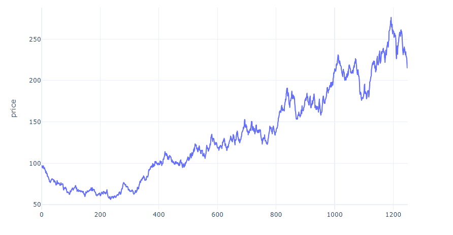
Figure (a) and Figure (b) show examples of the two methodologies. In the first case, the protection grows over time at a fixed rate as:
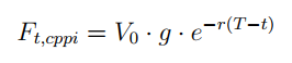
In the second case, the floor adjusts upwards to maintain the same level protection with respect to the portfolio value at each point in time t:
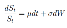
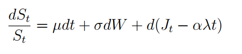
Now that we have explained the difference between the two approaches we focus on the statistical properties of TIPP. To do that, we follow the methodological approach used for CPPI by Khuman et al. (2008) and implement the same analysis to this new technique. In particular, we investigate the behavior of our risk metrics obtained by applying TIPP on two simulated processes: Geometric Brownian Motion (GBM) and Jump Diffusion Process (JDP). These processes represent a proxy for our risky financial assets. Given that we set an expected negative jump size to reflect the negative skewness of financial markets, we allow for fair comparison between the two processes by introducing a positive compensator to the JDP.
To validate the effectiveness of the strategy under two scenarios, we consider four relevant risk metrics:
- Average Final Payoff
- Probability of Gap i.e. a floor breach
- Excess Sharpe Ratio
- Maximum Drawdown
RESULTS
The first analysis aims to understand the properties of TIPP when the multiplier (m) and the rebalancing frequency (n) are let vary. The below table shows the multidimensional structure for our measures of interest.
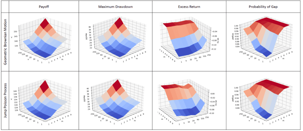
In general, the introduction of negative market jumps reduces by 10% on average the final payoff and increases the likelihood of a floor violation by 2-4%. For low multipliers and frequent rebalancing, the graph shows similar values of maximum drawdown. In this case, the presence of jumps does not impact the results significantly. Conversely, a 3% higher drawdown can be seen at the top of the surface when the jump is added. In terms of Sharpe ratio, the table indicates a strong preference for low exposure and daily rebalancing. In accordance with our initial intuition, higher m increases volatility more than what it does on performance. Considering the capital protection peculiarity of the TIPP and the impact of m on volatility and transaction costs, we believe that setting a multiplier in a 2 to 4 range would considerably benefit the implementation and monitoring of such approach.
Then we investigate the impact of transaction costs and turnover effect. Given the more volatile nature, the transaction fees incurred in the case of JDP will always exceed those paid in the GBM scenario. For this reason, we will conduct our analysis for the JDP case only. Management fees are not included in this case.
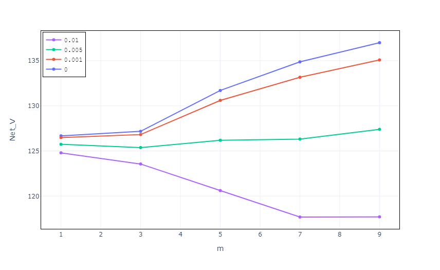
As the percentage fee increases, the final portfolio value falls exponentially. In particular, for the case of tc = 0.001, the net payoff is not significantly altered compared to the zero fee case. In contrast, we see a substantial impact for m ≥ 4 and higher transaction costs. For m = 9, only a -10% risk asset weekly return would result in a full portfolio rebalance from maximum (120) to minimum (40) exposure.
CONCLUSION
The result of the study reveals that the strength of TIPP varies significantly across the two stochastic processes. The model was better able to mitigate losses in the GBM compared to the JDP case, indicating a high sensitivity to the risky asset return distribution. Moreover, we saw that high volatility and transaction costs impair the usage of multipliers above 5 and that, to increase the exposure and avoid stalling, investors in TIPP could set a lower bound of minimum level of risky asset to be hold in the portfolio instead. Conversely, increasing leverage does not have positive results on performance. Finally, we highlight how having a cost efficient trade execution represents a major constraint for TIPP fund managers, with that aspect becoming increasingly important for more aggressive funds.
Authors:
Gianluca Baglini, Baglini Finance
Tony Berrada, University of Geneva
Are you looking for more strategies to read about? Sign up for our newsletter or visit our Blog or Screener.
Do you want to learn more about Quantpedia Premium service? Check how Quantpedia works, our mission and Premium pricing offer.
Do you want to learn more about Quantpedia Pro service? Check its description, watch videos, review reporting capabilities and visit our pricing offer.
Do you want algorithmic access to the full Quantpedia database via the API? Subscribe to Quantpedia Pro, ask for an API key, and explore the in/out-of-sample statistics, source academic papers, and code snippets — ideal for quantitative research, systematic trading workflows, and AI model training.
Are you looking for historical data or backtesting platforms? Check our list of Algo Trading Discounts.
Or follow us on:
Facebook Group, Facebook Page, Telegram, Twitter, Linkedin, Medium or Youtube
Share onLinkedInTwitterFacebookRefer to a friend


