Why Mean-Variance Optimization Breaks Down

Mean-Variance Optimization remains the intellectual cornerstone of modern portfolio theory, yet its real-world deployment via plug-in MVO often delivers unstable, over-leveraged portfolios that collapse out-of-sample. The core insight from VertoxQuant’s analysis is profound: raw plug-in MVO does not merely propagate estimation error—it systematically amplifies it. This error-maximization phenomenon occurs because the optimizer’s inverse-covariance operator assigns extreme weights to directions that appear low-risk, which, in finite samples, are dominated by noise rather than signal. For academics, this reveals a fundamental statistical pathology; for practitioners, it explains why backtests sparkle while live portfolios bleed.

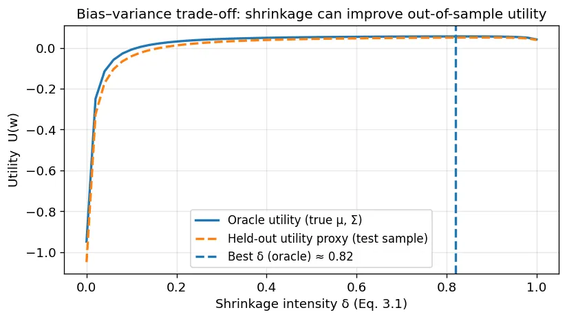
The solution requires a disciplined two-pronged approach targeting both inputs and the optimization process. Input regularization techniques deliberately introduce structured bias to stabilize noisy estimates: shrinkage pulls sample covariances toward well-conditioned targets, factor models impose economic structure to reduce dimensionality, and the Black-Litterman framework anchors expected returns to equilibrium priors, preventing the optimizer from chasing spurious alpha. These methods don’t eliminate uncertainty—they manage it intelligently, trading modest bias for dramatically lower out-of-sample weight variance. Empirical simulations confirm that even modest regularization can improve out-of-sample utility by over 100%, transforming fragile theoretical portfolios into implementable strategies.

Equally critical are optimizer constraints that restrict the solution space to prevent noise-driven extremes. Ridge/LASSO penalties shrink extreme parameter estimates and encourage sparsity; robust optimization hedges against worst-case parameter deviations by optimizing over uncertainty sets; and turnover penalties align rebalancing frequency with transaction cost realities. When combined with regularized inputs, these constraints produce portfolios that are stable, implementable, and resilient to estimation noise. The takeaway for both researchers and practitioners is clear: robust Mean-Variance Optimization isn’t about finding perfect estimates—it’s about engineering decision rules that perform well under uncertainty. By respecting the statistical realities of financial data and deliberately regularizing both inputs and the optimizer, we can finally make MVO work in the real world.

Authors: Vertox

Title: Why Mean-Variance Optimization Breaks Down

Link: https://www.vertoxquant.com/p/why-mean-variance-optimization-breaks

Abstract:

Mean–Variance Optimization (MVO) is a central framework for portfolio construction: choose weights that balance expected return against risk as measured by variance.

In its classical form, MVO is elegant, convex (under mild conditions), and analytically tractable. Yet practitioners quickly encounter a paradox: the mathematically “optimal” portfolio built from estimated inputs is often unstable, highly leveraged (explicitly or implicitly), and disappoints out-of-sample.

This is not a minor implementation detail; it is a structural consequence of combining a high-dimensional optimizer with noisy estimates of expected returns and covariances.

This article develops MVO from first principles and then explains, in a mathematically explicit way, why raw MVO tends to maximize estimation error.

Finally, it surveys the spectrum of practical fixes, organized around two levers: (i) improving or regularizing the inputs (expected returns and covariances), and (ii) constraining or regularizing the optimizer (the feasible set and the objective).

The unifying theme is that almost every successful “fix” works by injecting bias in exchange for a large reduction in variance of the resulting portfolio weights, thereby improving out-of-sample performance and implementability.

As always, we present several interesting figures and tables:

Notable quotations from the academic research paper:

“When raw MVO meets real data, the mathematical mechanisms above manifest in operational ways:

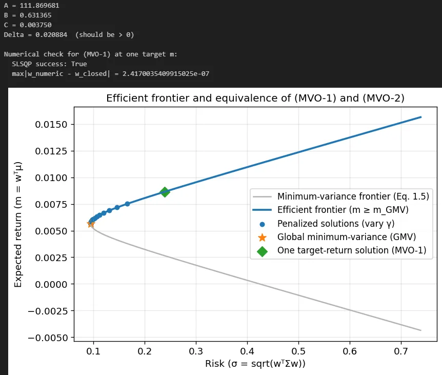
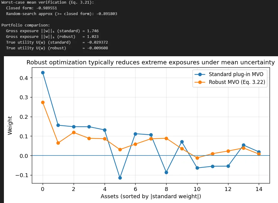
• Extreme weights and implicit leverage. Even with the budget constraint 1^T w = 1, weights can be large positive and large negative (if shorting is allowed), producing large gross exposure |w|_1. Even with no-short constraints, solutions often sit on corners of the feasible region (many weights at bounds), because linear return objectives push to extremes.

• High sensitivity to small input changes. Updating the estimation window by one month can materially change hat{mu} and hat{Sigma}, leading to large changes in hat{w}. This is not merely “rebalancing”; it is model instability.

• High turnover and transaction cost drag. If weights change drastically, realized performance is dominated by trading costs and market impact, neither of which exists in the clean Markowitz formulation unless explicitly modeled.

• Out-of-sample underperformance relative to naive allocations. A simple equal-weight or risk-parity portfolio can outperform a naive MVO portfolio after costs, not because those heuristics are theoretically superior, but because they are robust to estimation error.

These observations motivate the central practical conclusion: raw plug-in MVO is a high-variance estimator of portfolio weights. In modern terms, it is an overfit model.

If raw MVO is fragile because it optimizes a noisy objective with unstable operators, then fixes must do one (or both) of the following:

1. Fix the inputs: replace (hat{mu}, hat{Sigma}) with estimators that have lower estimation error, better conditioning, or an economically grounded structure.

2. Constrain or regularize the optimizer: modify the optimization problem so that it cannot translate small input errors into extreme weight changes.

These approaches are complementary. Many production-grade systems use both: structured/shrunk inputs and a constrained, regularized optimization.

Before invoking the next equation, it helps to distinguish between two regimes:

• Risk-free asset (tangency portfolio). If a risk-free asset is available and w_m is the tangency portfolio, then pi are excess returns and reverse optimization yields pi = lambda Sigma w_m.

• Risky-only, fully invested. If we remain in the 1^T w = 1 setting, the KKT condition is mu = gamma Sigma w_m + eta 1. The intercept term is economically irrelevant under the budget constraint, so one can normalize it away or interpret eta as the baseline rate.

It is tempting to treat the practical modifications above as an ad hoc toolbox: shrinkage here, constraints there, turnover penalties elsewhere. A more coherent view is that these methods all solve the same underlying problem:

The plug-in MVO portfolio is a high-variance estimator of the optimal weights.

Reducing that variance requires injecting structure, equivalently, adding bias.

• Shrinkage of Sigma reduces the variance of covariance estimates (and stabilizes inversion) at the cost of bias toward the target structure.

• Factor models impose a low-rank structure that may be misspecified but dramatically reduces estimation noise.

• Shrinkage and Bayesian methods for mu explicitly acknowledge that sample means are too noisy to trust fully.

• Constraints and penalties reduce the effective degrees of freedom of the portfolio, preventing the optimizer from encoding noise into intricate weight patterns.

• Turnover penalties reduce the variance of changes in weights, which is often the real operational pain point.

• Robust optimization is an explicit uncertainty-aware form of regularization.

From this perspective, the “right” portfolio is not the one that is optimal for the estimated parameters; it is the one that is optimal for the decision problem under uncertainty, including estimation error, non-stationarity, and implementability constraints.”

Are you looking for more strategies to read about? Sign up for our newsletter or visit our Blog or Screener.

Do you want to learn more about Quantpedia Premium service? Check how Quantpedia works, our mission and Premium pricing offer.

Do you want to learn more about Quantpedia Pro service? Check its description, watch videos, review reporting capabilities and visit our pricing offer.

Do you want algorithmic access to the full Quantpedia database via the API? Subscribe to Quantpedia Pro, ask for an API key, and explore the in/out-of-sample statistics, source academic papers, and code snippets — ideal for quantitative research, systematic trading workflows, and AI model training.

Are you looking for historical data or backtesting platforms? Check our list of Algo Trading Discounts.

Or follow us on:

Facebook Group, Facebook Page, Telegram, Twitter, Linkedin, Medium or Youtube