2-Year Notes Momentum: Extracting Term Structure Anomalies from FOMC Cycles
Introduction
For many investors, short-term interest rates are often treated as something the market “discovers.” In reality, the Federal Reserve has enormous control over how the front end of the yield curve evolves. While textbooks often portray the Fed’s policy rate as a flexible tool that reacts quickly to economic data, the actual behavior of the Federal Open Market Committee (FOMC) looks very different. In practice, monetary policy tends to move in long, persistent cycles. The Fed spends years hiking rates, or years cutting them, and only rarely reverses direction quickly. For anyone trading rates, bonds, or rate-sensitive assets, this persistence matters. It means that the path of short-term interest rates over the next one to two years is often largely shaped by the Fed’s policy trajectory rather than by constantly shifting market expectations.
This observation has an important implication: the short end of the Treasury curve often behaves less like a forecasting market and more like a gradual reflection of the Fed’s policy cycle. When the Fed enters a tightening or easing phase, that trend tends to propagate through Treasury yields from one month out to roughly two years. In this article, we show that these policy-driven trends can be measured and used. By identifying whether the Fed is in a tightening, easing, or neutral phase, investors can improve their expectations about the near-term evolution of the yield curve. For fixed-income portfolio managers and macro traders, recognizing these policy regimes can help sharpen rate forecasts, improve duration positioning, and better manage risks tied to interest-rate movements.
Background
The Federal Reserve has unusually strong influence over the shortest part of the yield curve because of the way modern monetary policy is implemented. Under the current “ample reserves” system, the Fed guides overnight interest rates mainly through two administered tools: the Interest on Reserve Balances (IORB) and the Overnight Reverse Repurchase (ON RRP) facility, which effectively set a floor for money-market rates (Ihrig, J. E., Meade, E. E., & Weinbach, G. C. (2015)). In practical terms, this framework gives the Fed substantial control over interest rates from overnight maturities out to roughly the 2-year horizon. Beyond that point, other forces—such as inflation expectations, term premia, and global capital flows—play a much larger role. The key takeaway for investors is that the front end of the Treasury curve is not purely a market-driven forecasting mechanism. Instead, it largely reflects the Fed’s policy trajectory. We refer to this idea as the policy control dominance hypothesis: over shorter horizons, the path of rates is strongly anchored by the Fed’s own policy decisions.
Looking at past rate cycles makes this dynamic clear. Once the Fed begins tightening policy, rate hikes tend to continue across many meetings and often over several years. Easing cycles show a similar pattern in the opposite direction. This gradual approach is consistent with the central banking literature. Because policymakers face uncertainty about the economy and know that policy works with long and variable lags, they typically adjust rates cautiously to avoid abrupt reversals (Woodford, M. (2003)). Clarida, R., Galí, J., & Gertler, M. (2000) formalize this behavior with policy rules that include interest rate smoothing, meaning that central banks tend to adjust rates gradually toward their desired level. In practice, however, this smoothing is not constant. During a tightening or easing cycle, policy tends to move persistently in one direction, while the turning points between cycles can be abrupt. The result is that short-term rates often behave like a slow-moving trend within a policy regime, rather than a simple mean-reverting process.
Our contribution focuses on the practical implications of this behavior. We show that the persistence created by these multi-year Fed policy cycles—whether tightening, easing, or holding steady—creates trends that can be detected directly in 2-year Treasury futures prices. Importantly, exploiting this effect does not require building a complex macro model, identifying policy regimes in advance, or forecasting economic data releases. Instead, simple trend-following signals applied to futures prices naturally capture the same persistence embedded in Fed policy. In other words, rather than trying to predict the policy cycle first and then forecast rates, we let price momentum act as a filter that automatically adapts to the prevailing environment.
This perspective reframes how investors think about predictability at the front end of the yield curve. What might appear to be forecasts driven by macro surprises or market microstructure effects may, in part, simply reflect the slow and deliberate way the Federal Reserve adjusts policy over time. By using price-based signals, traders can capture this dynamic directly—without relying on subjective interpretations of the policy cycle.
Methodology
Instrument Selection and Leverage Rationale
We employ the CME 2‑Year Treasury Note futures contract (TU1) as our primary and only trading vehicle. This instrument is uniquely suited to capture the Federal Reserve’s directional influence on the short end of the yield curve: its pricing kernel is concentrated in the one‑ to two‑year maturity bucket, precisely where FOMC control is most direct and persistent. Longer-tenor futures, such as 10‑ or 30‑year futures, are contaminated by inflation expectations and global term premia, making them inferior for isolating policy‑driven trends. Critically, we utilise futures rather than cash ETFs because futures embed substantial implicit leverage through low margin requirements, allowing us to magnify the modest absolute returns inherent to front‑end fixed income. This leverage is not merely convenient but necessary—without it, the unconditional volatility of 2‑year yields is too low to generate economically meaningful returns.
We use continuously adjusted futures series constructed via the backward‑ratio roll methodology described in the next subsection. Our empirical analysis spans from July 1990 to January 2026. Although the underlying futures prices are available at a daily frequency, we sample end‑of‑month (EOM) observations to align with the typical rebalancing cycle of systematic trend strategies and to mitigate microstructure noise. All strategies assume execution at the closing prices.
Continuous Futures Construction
A robust backtesting framework for futures strategies must address the mechanical discontinuities that arise when rolling from an expiring contract to the next. Naïve splicing of contract prices creates artificial jumps that, if levered, produce entirely spurious performance signals. We therefore adopt the industry‑standard methodology for rolling:
Our continuous series is constructed using a first‑of‑month roll date, at which we exit the front contract and enter the first back contract. To eliminate the resulting price gap, we apply a backward-ratio adjustment: each historical contract price is multiplied by the ratio of the back‑month price to the front‑month price on the roll date. This approach preserves the percentage‑change representation of returns, ensures that the current contract price remains unaltered, and avoids the recalculation instability of additive methods. All empirical analysis reported in this study is performed on these rolled-ratio futures, ensuring that our performance metrics reflect genuine tradable outcomes rather than data‑construction artifacts.
Benchmarks & Reporting on Evaluation of Findings
As a baseline, we employ a passive long‑only position in the continuous 2‑year Treasury futures contract. The benchmark is implemented with a one‑month skip at the sample’s inception to eliminate any initialisation bias; thereafter, the position is held continuously. This passive strategy reflects the unconditional risk premium embedded in the short end of the curve and serves as the reference against which all active rules are evaluated.
Following, establish some practices and conventions to move our reporting forward. We report results before transaction costs to establish an upper bound. Visualizing equity curves provides a graphical view of capital appreciation and depreciation over time. Furthermore, we compute five standard performance and risk measures as in Portfolio Analysis, all expressed on an annualised basis:
Performance (p.a.) – geometric mean return.
Volatility (p.a.) – annualised standard deviation of returns.
Sharpe Ratio – using a 0% risk‑free rate.
Maximum Drawdown – peak‑to‑trough decline over the sample.
Calmar Ratio – annualised return divided by maximum drawdown.
And here, the promised equity curve of our passive benchmark, buy & hold of bond futures:
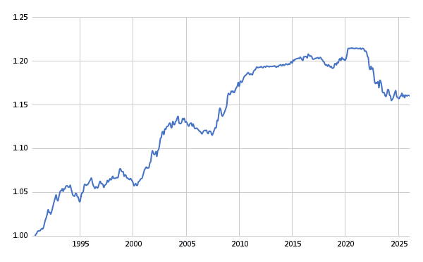
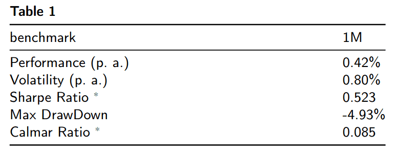
The passive long‑only benchmark, constructed from the continuous 2‑year Treasury futures series exhibits the modest return profile characteristic of front‑end fixed income. As illustrated in Figure 1, the cumulative equity curve advances slowly from a base of 1.00 in 1994 to 1.16 by 2025, corresponding to an annualised geometric return of approximately 0.42%. Volatility remains subdued throughout the sample, yet the strategy is not immune to drawdowns: the most pronounced decline occurs between 2021 and 2023, when the cumulative value retreats from 1.22 to 1.16—a peak‑to‑trough loss of roughly 5%. Consequently, the benchmark delivers a Sharpe ratio (0% risk‑free rate) of around 0.5 and a Calmar ratio below 0.1 across the full evaluation period. These risk‑adjusted returns set a stringent baseline: any active rule must deliver economically meaningful outperformance to be considered non‑trivial.
Signal Construction: A Trend-Following Framework
From this continuous futures series, we extract directional signals using a suite of canonical trend-following indicators. Specifically, we employ conventional momentum (MOM) indicators defined on cumulative returns over formation periods: first, the rate-of-change (ROC) and second, the simple moving average (SMA) specifications across multiple lookback windows. These specifications are deliberately standardized; our contribution lies not in signal innovation but in applying these ubiquitous tools to a market segment—the short end of the Treasury curve—to test persistent directional drift. The institutional regularity we describee in the previous section—protracted FOMC hiking and easing cycles spanning multiple years—implies that 2-year yields should exhibit precisely the sort of serial dependence that trend rules are designed to exploit. By conditioning on nothing more than the futures price history itself, our approach remains free of subjective regime-classification heuristics. This parsimony is intentional: we establish that even the most elementary trend-following rules generate economically meaningful risk-adjusted returns in this arena. The implication is not that market participants irrationally neglect Fed communications, but rather that the degree of policy persistence is itself underestimated by the yield curve’s consensus expectations.
Results
We evaluate two families of momentum indicators, each computed from the continuous futures series and updated monthly.
Trend‑Following Signals Specifications
For each rule, we report three implementations:
Long‑only – long when the long condition holds (e. g., the current price exceeds the moving average), otherwise flat.
Short‑only – short when the short condition holds (e. g., the current price is below the moving average), otherwise flat.
Long‑short – long when the long condition holds and short when the short condition holds; flat when neither or both conditions are met (the latter never occurs by construction).
Rate‑of‑Change (ROC)
Trading rules for lookback windows 1, 2, 3, 6, 9, 12, and 24 months go as follows:
- A long position is taken when the cumulative return across the one indicated lookback window is positive.
- A short position is taken when the cumulative return across the one indicated lookback window is negative.
Simple Moving Average (SMA)
For each lookback window w ∈ {2, 3, 4, 5, 6, 9, 12, 24} months, we compute the trailing moving average of end-of-month prices and apply the previously mentioned universal rulesets.
Empirical Findings
Figures 2, 3, and 4 display cumulative equity curves of each ROC strategy variant.
Tables 2, 3, and 4 report previously established evaluation metrics for each ROC specification.
Figures 5, 6, and 7 establish equity curves for SMA strategy types, and Tables 5, 6, and 7 present reported results for SMA strategy variations.
Each is accompanied by a short commentary to establish ideas and insights before final discussions and conclusions.
Long‑only ROC
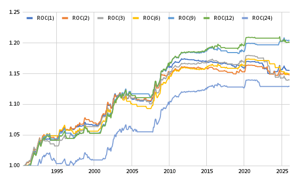
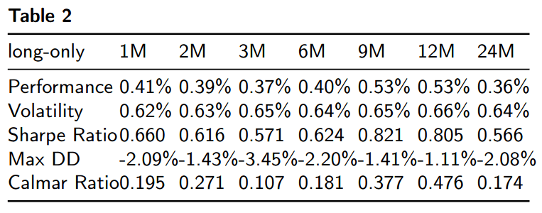
All rate‑of‑change lookback windows generate positive cumulative equity curves over the sample period, with terminal values of 9M and 12M uniformly exceeding the passive benchmark’s final value of 1.16, indicating that systematic long exposure conditioned on unanimous positive momentum across multiple horizons systematically outperforms a static long position. Performance is not uniform across windows: longer formation periods (9, 12, and 24 months) produce higher cumulative returns and exhibit smoother equity appreciation, whereas shorter windows (1–3 months) deliver more moderate gains. Consistent with the discussion in the last section, each long‑only ROC specification improves upon the benchmark’s Sharpe and Calmar ratios, confirming that the directional persistence of FOMC cycles is reliably captured by even the simplest trend‑following filters.
Short‑only ROC
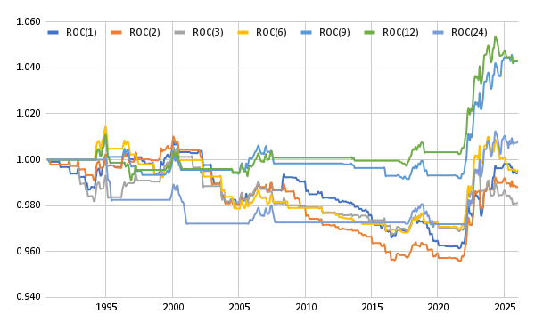
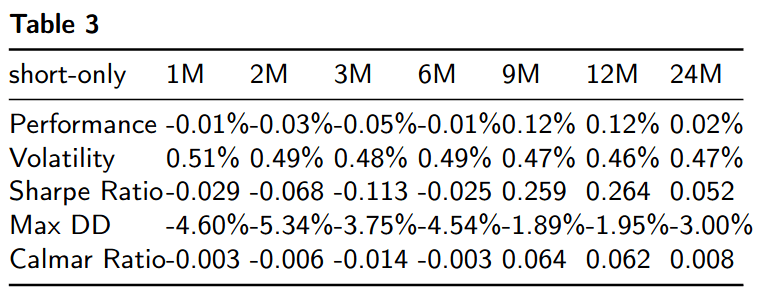
In contrast, every short‑only ROC rule produces cumulative equity values below unity throughout the sample, with terminal values concentrated between 0.98 and 1.05. The persistent downward drift reflects the prolonged secular decline in yields and the associated upward trajectory of Treasury futures prices over most of the 1995–2022 period. Unconditional short exposure therefore destroys value, and the negative Sharpe ratios obtained across most lookback windows serve as a useful falsification test: the predictability we document is not symmetric, but rather aligned with the Fed’s historical bias in the last 30 years toward accommodation and the resulting positive drift in front‑end prices.
Long‑short ROC
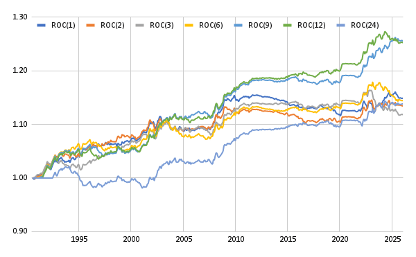
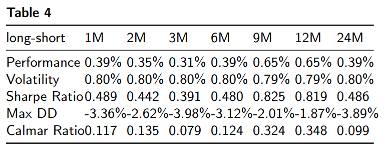
The long‑short implementations combine the long and short entry rules to maintain directional neutrality while preserving exposure to cyclical turning points. Cumulative equity curves exhibit consistent growth across all lookback horizons, with some terminal values exceeding those of the corresponding long‑only rules—reaching approximately 1.27 for the 9‑ and 12‑month specifications by 2025. However, the Calmar ratios are slightly decreased relative to both the benchmark and the long‑only variants, reflecting sharper, though still shorter-lived, drawdowns. For intermediate lookbacks (9–12 months), Sharpe ratios surpass those of the long‑only versions by a bit. These findings confirm that an investor seeking to neutralise the prevailing drift bias can do so without sacrificing profitability; indeed, the long‑short formulation extracts additional performance from correctly identified regime reversals while hedging against the sustained upward trend that dominates unconditional returns.
Long‑only SMA
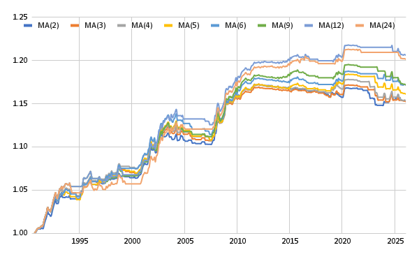
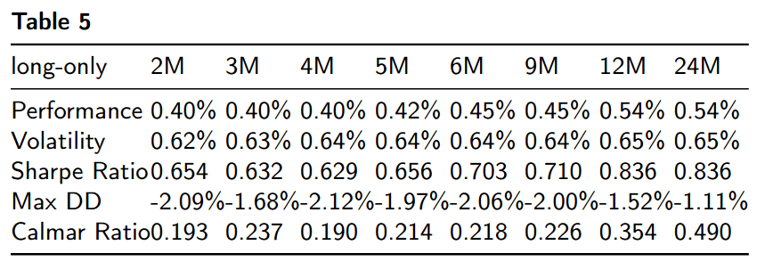
Longer (than five months) moving‑average lookback windows generate positive cumulative-equity curves that consistently outperform the passive benchmark. Terminal values by 2025 range from approximately 1.15 to 1.22, with longer formation periods (12 and 24 months) exhibiting higher peak equity earlier in the sample before modest mean reversion. Intermediate windows (6–9 months) deliver the smoothest appreciation and the most favourable risk‑return trade‑off, as evidenced by Sharpe ratios consistently exceeding 0.5 and Calmar ratios double that of the benchmark. The long‑only SMA rules thus provide robust, systematic exposure to the directional persistence of Fed policy cycles, confirming that simple trend-detection in the 2‑year futures market yields economically meaningful outperformance.
Short‑only SMA
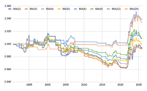
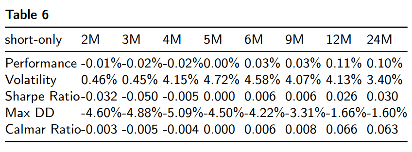
In contrast, unconditional short exposure conditioned on price‑below‑moving‑average signals produces sustained losses across most lookback windows. Cumulative equity for windows of 2, 3, 4, and 6 months remains persistently below unity, with terminal values near 1 and maximum drawdowns exceeding 4%. Longer lookbacks (12 and 24 months) show brief intervals of profitability during cyclical downturns but ultimately deliver negligible or negative full‑sample returns.
Long‑short SMA
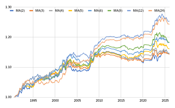
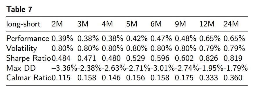
Combining the long and short entry rules neutralises the prevailing drift while preserving exposure to genuine cyclical reversals. Cumulative equity curves exhibit consistent, monotonic growth across all lookback horizons, with terminal values exceeding 1.20 for intermediate windows and approaching 1.27 for the 12‑ and 24‑month rules. Longer lookbacks (12 and 24 months) thus produce even more pronounced appreciation, reflecting their ability to capture extended policy cycles with fewer false signals. Crucially, those long‑short implementations deliver Calmar ratios that are materially higher than both the benchmark and the corresponding long‑only variants, confirming that drawdowns are shallower and recoveries faster. For windows of 6 to 12 months, Sharpe ratios also surpass those of the benchmark and some long‑only specifications. These results establish that an investor seeking to remain directionally neutral—neither structurally long nor short the front end—can nonetheless extract substantial risk‑adjusted returns by systematically following the trend signals embedded in the FOMC’s own policy cadence.
Discussion and Conclusions
These findings confirm that elementary, purely price‑based trend signals systematically extract value from the 2‑year Treasury futures market. The robustness of the results across multiple lookback windows and implementation variants underscores that the documented predictability is a direct, reduced‑form manifestation of the Federal Reserve’s inertial policy cycles.
This paper provides systematic evidence that the Federal Reserve’s inertial policy cycles imprint a persistent, exploitable directional component on the front end of the US Treasury yield curve. Using only the price history of 2‑year note futures, we demonstrate that elementary trend‑following rules—both rate‑of‑change and moving‑average specifications—generate statistically and economically significant excess returns over a 35‑year sample. These findings carry two principal implications.
First, the long‑only versions of longer-timespan momentum and moving‑average rules substantially outperform the passive benchmark on a risk‑adjusted basis. Annualised Sharpe ratios exceed those of the benchmark by a wide margin, and Calmar ratios are uniformly improved. The magnitude and persistence of these excess returns suggest that the directional drift embedded in FOMC policy cycles is consistently underestimated by market participants. In effect, the yield curve’s consensus expectation of the future short rate path is systematically too flat relative to the actual persistence of Fed tightening and easing cycles.
Second, the long‑short implementations offer a directionally neutral alternative that preserves the economic gains while removing reliance on the secular decline in yields. Across longer-windowed ROC and SMA specifications, the long‑short variants deliver higher annualised returns and superior Calmar ratios relative to both the benchmark and their long‑only counterparts. For intermediate lookback windows, long‑short Sharpe ratios also exceed those of long‑only strategies. This pattern is crucial for two reasons. It confirms that the predictability we document is not merely a reflection of the unconditional term premium or a one‑sided bull market; rather, it arises from genuine cyclical turning points. Moreover, it provides institutional investors—who may be constrained from expressing persistent directional views—with a viable, bias‑neutral implementation that remains firmly grounded in observable futures-price history.
Several limitations warrant acknowledgment. Our analysis deliberately omits transaction costs to establish an upper bound on performance; while turnover is modest, a full implementation would need to account for bid‑ask spreads and market impact, particularly during periods of elevated volatility. Additionally, our signals are re‑evaluated monthly; daily implementations might capture turning points more promptly but would incur higher trading frictions. Future research could extend this framework along multiple dimensions: incorporating option‑implied information to refine entry and exit timing, testing the strategy across other tenors where Fed influence is attenuated but still present (e.g., 5‑year notes), or developing structural models that explicitly link the optimal control problem of the central bank to the trend‑statistics we employ.
In conclusion, this paper establishes that the directional persistence inherent in Federal Reserve policy cycles is not merely a descriptive curiosity of monetary economics—it is a robust, tradeable anomaly in the very asset class the Fed most directly influences.
Author: Cyril Dujava, Quant Analyst, Quantpedia
Are you looking for more strategies to read about? Sign up for our newsletter or visit our Blog or Screener.
Do you want to learn more about Quantpedia Premium service? Check how Quantpedia works, our mission and Premium pricing offer.
Do you want to learn more about Quantpedia Pro service? Check its description, watch videos, review reporting capabilities and visit our pricing offer.
Are you looking for historical data or backtesting platforms? Check our list of Algo Trading Discounts.
Or follow us on:
Facebook Group, Facebook Page, Twitter, Linkedin, Medium or Youtube
Share onLinkedInTwitterFacebookRefer to a friend