Would you like to see the performance of your portfolio 100 years back in history? Do you want to analyze the risk of your strategy under 100 years of real historical scenarios? All of these, and much more, will be soon (in a few days) available for Quantpedia Pro subscribers. How? We will explain today how we can model a 100-year history of your portfolio.
Replicating Portfolios with Factors
When reading the title of this article, the first question that might come to your mind is why would anyone want to replicate a portfolio with risk factors. Nevertheless, there are many reasons why replicating a portfolio with factors is beneficial.
For example, as ETFs were only developed in the 1990s, only very limited historical time windows are available to analyze their performance in extreme market conditions. Also, many strategies rely on ETFs, so their histories are usually only 20 years long, often much shorter. Having the ability to replicate any portfolio with factors with longer history might provide us with countless valuable information.
Another reason for replicating might be an interest in someone else’s portfolio. What factors drive my competitor’s returns? On the other hand, you might also want to find out to which factors is your own portfolio most sensitive. Whatever the case might be for you, having a more extended data history is always beneficial.
Therefore, we examined 20 factors and used them to replicate various portfolios in the following steps:
- In the first step, we synchronize the factor and portfolio dates to allow for further calculations.
- Secondly, we use multi-factor regression analysis in combination with Akaike’s Information Criterion (AIC) to find the explanatory factors of a portfolio and their weights. We apply the procedure to the available history of one’s input portfolio.
- Thirdly, we check our fit quality by visualizing equity curves of both the original and factor portfolios for the available history of an input portfolio.
- Lastly, we extend the history of a portfolio to 100 years by modelling an input portfolio via factors with rich data history, created based on Quantpedia’s unique methodology.
We will now dive deeper into the methodology in the following sections.
100 Years of Daily Factor Data
First of all, we had to choose carefully our factor universe – i.e. what will be our building block for modelling portfolios and strategies. In this choice we had to take into account both:
- Having enough uncorrelated and representative market factors for various asset classes
- Long-term Data availability for such underlying factors
However, finding factor data with a 100-year history is almost impossible. Thus, we had to get creative and produce our own data series. With the exception of a few factors, we combined multiple data sources to obtain historical data from 1926. We list the factors and a short description of the methodology for obtaining the data below.
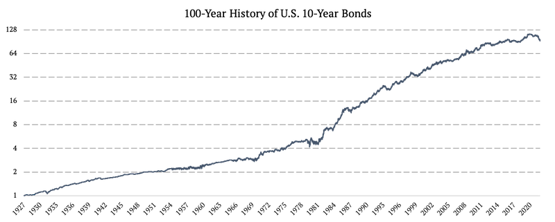
U.S. 10-Year Bonds (US10Y)
We described the process of creating a 100-year history of U.S. 10-Year Bonds in detail in our data primer: Extending Historical Daily Bond Data to 100 Years. To obtain the 100-year history, we combined three data sources:
1926 – 1962: Monthly US 10-Year Bond Yields
1962 – 2002: Daily US 10-Year Bond Yields
2002 – 2022: IEF ETF (iShares 7-10 Year Treasury Bond ETF)
From 1926 to 1962, we worked with monthly yields, and from 1962 to 2002, with daily yields. Firstly, we transformed the bond yields into total returns. Once we calculated the returns, the second challenge was to transform the monthly returns from 1926 to 1962 into daily ones.
We achieved that by extrapolating the daily volatility from the US 3-month T-bills, our unique method we call a “Volatility proxy extrapolation”. In simple terms, we copy the daily volatility from the 3-month T-bills, and plug it in between two monthly data points of US 10-year Treasuries.
As mentioned above, this is only a short summary of the methodology. If you are interested in the specific details of any of the steps, please see Extending Historical Daily Bond Data to 100 Years.
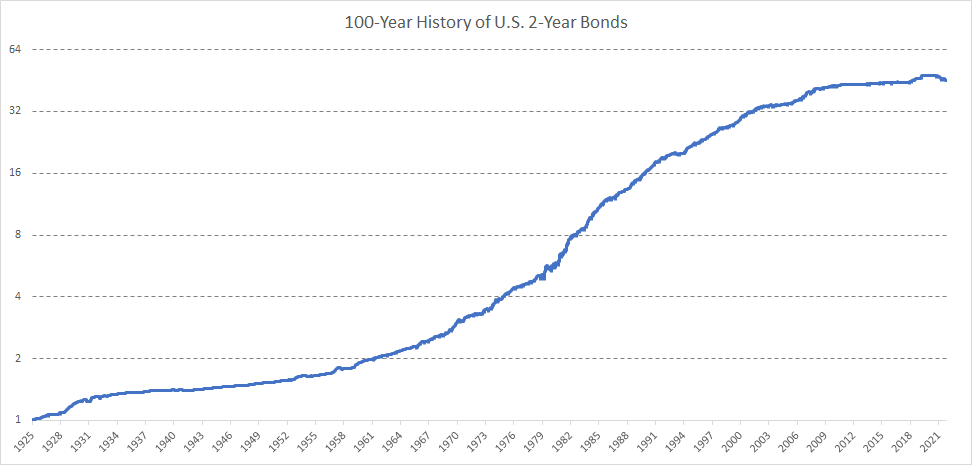
U.S. 2-Year Bonds (US2Y)
Accordingly to the methodology for the US 10-year bonds, we created 100-year history also for 2-year bonds. We combined the following sources:
1926 – 1934: we used monthly 3M rates and monthly 5y rates, interpolated 2y yield and interpolated daily price series from 2y rate
1934 – 1940: we used monthly 3M dealers and 3-5y Notes monthly data, interpolated 2y yield and interpolated daily price series from 2y rate (https://fraser.stlouisfed.org/title/banking-monetary-statistics-1914-1941-38/part-i-6408) pages 460-462
1941 – 1962: we used 9-12M issues market yield a 3-5y issues, interpolated 2y yield and interpolated daily price series from 2y rate (https://fraser.stlouisfed.org/title/banking-monetary-statistics-1941-1970-41) pages 697-703,
1962 – 1976: we interpolated daily 2y yield from 1y/5y daily rates from FRED and calculated price series
1976 – 2002: we used daily data from FRED (https://fred.stlouisfed.org/series/DGS2)
2002 – 2022: SHY ETF (iShares 1-3 Year Treasury Bond ETF)
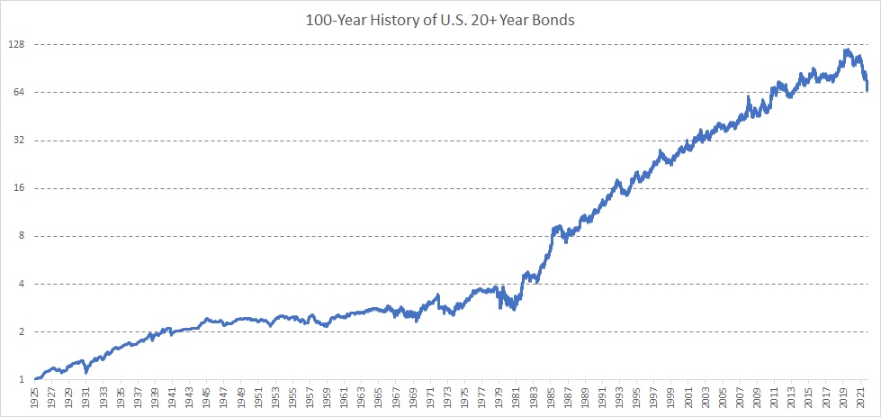
U.S. 20+ Year Bonds (US20Y)
Again, accordingly to the methodology for the US 10-year bonds, we created 100-year history also for 20+ year bonds. We combined the following sources:
1925 – 1941: we used 10-year yield as proxy with a duration fitting 25y bonds (as TLT ETF has) + we then interpolated monthly data to daily
1942 – 1961: we used 20-year yield from FRED (https://fred.stlouisfed.org/series/M13058USM156NNBR), then extrapolated 25-yield yield from 10y a 20y, created price series with duration fitting 25y bonds + we then interpolated monthly data to daily
1962 – 1976: we used 20-year yield from FRED (https://fred.stlouisfed.org/series/DGS20), then extrapolated 25-yield yield from 10y a 20y, created price series with duration fitting 25y bonds + we then interpolated monthly data to daily
1976 – 1986: we used 30-year yield from FRED (https://fred.stlouisfed.org/series/DGS30), then extrapolated 25-yield yield from 20y a 30y, created price series with duration fitting 25y bonds + we then interpolated monthly data to daily
1987 – 1993: daily price data calculated from 25-y yield interpolated from 10-y and 30-y daily yields
1993 – 2002: daily price data calculated from 25-y yield interpolated from 20-y and 30-y daily yields
2002 – 2022: TLT US (iShares 20+ Year Treasury Bond ETF)
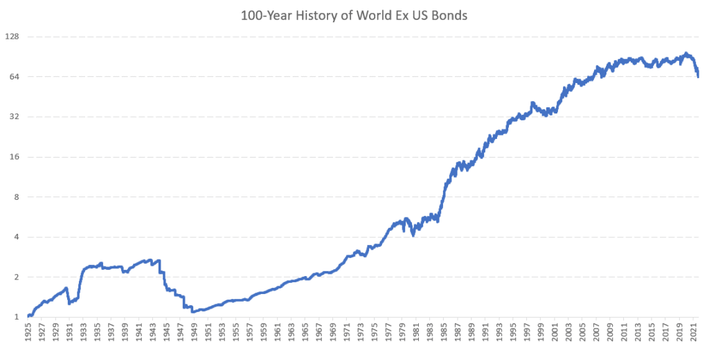
World Ex US Bonds
To obtain a 100-year history of World Ex US Bonds, we combined the following data sources:
1926 – 1980: we used monthly data from FRED on the 10-year yield of the following countries – UK, GER, JAP, FRA, ITA, NET, CAN, AUS, CHINA, KOREA, and GDP-weighted them into the synthetic 10-year ex-US yield. Countries were added to the portfolio as the data became available. We then interpolated monthly data into daily and created a total return price series. That price series was then converted into the USD currency by using our data series on the dollar factor.
1980 – 2007: we used the same methodology as for the 1926-1980 period, but this time, we do not need to perform interpolation as sufficient daily yield data are available.
2007 – 2022: BWX US (SPDR® Bloomberg International Treasury Bond ETF)
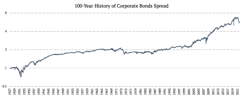
Corporate Bonds Spread (BAA CORP)
To obtain a 100-year history of Corporate Bonds, we combined the following data sources:
1926 – 1985: Monthly Baa Corporate Bond Yield
1986 – 2002: Daily Baa Corporate Bond Yield
2002 – 2022: spread between LQD ETF (iShares iBoxx $ Investment Grade Corporate Bond ETF) and IEF ETF (iShares 7-10 Year Treasury Bond ETF)
Similarly to U.S. 10-Year Bonds, we applied daily volatility proxy extrapolation to the monthly returns for the first data source. Only this time, we used the beta-adjusted equity market returns as the source of volatility. The beta was calculated so that the volatility of the equity market matched the volatility of bonds.
During first two periods, we had to again transform bond yields into total returns, in the same fashion as was the case with US Treasury yields described above. To better understand our entire data methodology, we advise reading Extending Historical Daily Bond Data to 100 Years.
Finally, we utilize the corporate bonds data in the form of a spread against US Treasuries. This way we are able to isolate the credit spread effect and include it separately, in addition to a “curve” effect represented by US Treasuries.
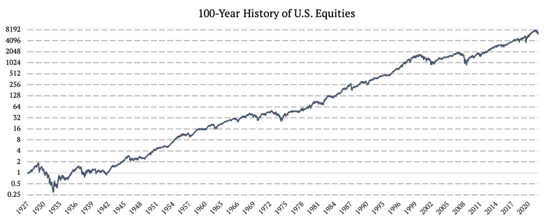
U.S. Equities (US EQUITIES)
The construction of the U.S. Equities factor was fairly straightforward. We simply combined Fama & French market factor (1926 – 1993) from Fama & French data library and SPY (SPDR S&P 500 ETF Trust) ETF’s daily returns (1993 – 2022).
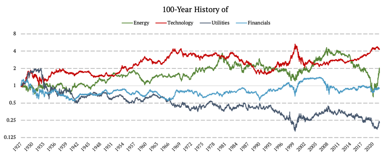
US Equity Sectors’ Spreads (Energy, Technology, Utilities, Financials)
The data for market factors were obtained from Fama & French data library specifically from the 12 Industry Portfolios [Daily]. We used:
- the spread of the Energy industry against the market as the Energy factor
- the spread of the Business Equipment industry against the market as the Technology factor
- the spread of the Healthcare, Medical Equipment, and Drugs against the market as the Health Care factor
- the spread of the Utilities industry against the market as the Utilities factor, and
- the spread of the Money industry against the market as the Financials factor.
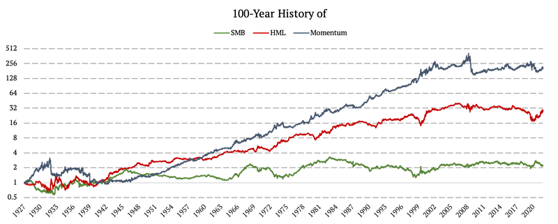
Fama & French Factors (SMB, HML, Momentum)
Similarly, we obtained data for Small-Minus-Big (SMB), High-Minus-Low (HML), and Momentum factors from Fama & French data library. However, no spreads were calculated for these factors – because they are already in the form of a long-short spread. The factors are available from 1926 to today.
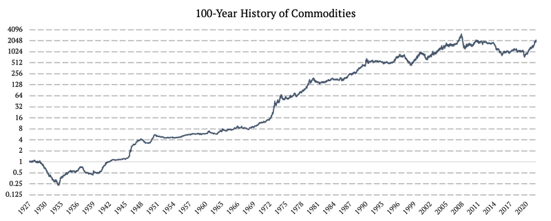
Commodities
The process of obtaining a 100-year history of commodity data is detailly described in Quantpedia’s data primer: Extending Historical Daily Commodities Data to 100 Years. We used three data sources:
1926 – 1979: Monthly PPI (Producer Price Index by Commodity: All Commodities)
1980 – 2006: S&P GSCI Commodity Total Return (SPGSCITR)
2006 – 2022: DBC ETF (Invesco DB Commodity Index Tracking Fund)
Firstly, between 1926 – 1979 we adjusted the PPI index to account for the correct commodity prices beta. Secondly, we used the excess return of the equity Energy sector vs. the entire market as our daily volatility proxy. We applied Quantpedia’s Volatility Proxy Extrapolation and obtained daily data from this monthly source.
If you are interested in the specific details of any of the steps, please see our article Extending Historical Daily Commodities Data to 100 Years.
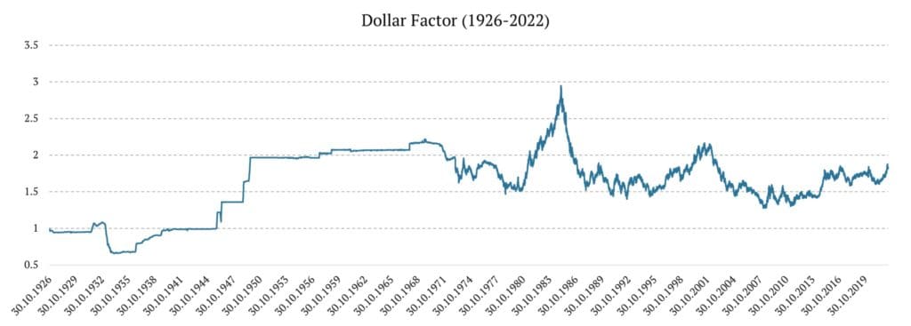
The US Dollar Factor
The US Dollar factor was constructed using 3 different data sources:
1926 – 1953: cross-currency rates were obtained from riksbank.se.
1953 – 1971: cross-currency rates were obtained from bis.org
1971 – 2007: we obtained Wikipedia’s U.S. Dollar Index
2007 – 2022: we use UUP ETF (Invesco DB US Dollar Index Bullish Fund)
The complete methodology is explained in the following article.
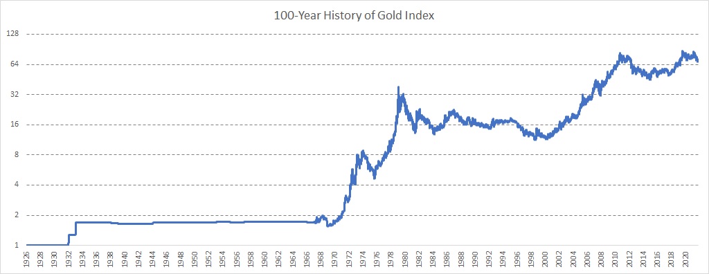
Gold
The Gold Index was constructed in three steps:
1926 – 1968: We used monthly Gold prices and linear interpolation to obtain daily Gold Index
1968 – 2004: We used daily spot Gold prices
2004 – 2022: GLD ETF (SPDR Gold Shares)
World Ex-US Equities Spread (WorldExUS)
The WorldExUS factor was constructed in several steps and utilized multiple data sources.
1926 – 1972: Monthly World ex-US equities
1972 – 2002: Daily World ex-US equities
2002 – 2007: EFA ETF (iShares MSCI EAFE ETF)
2007 – 2022: VEU ETF (Vanguard FTSE All-World ex-US Index Fund)
Similarly to the Bond data above, we applied Quantpedia’s volatility proxy extrapolation to transform the monthly data from the first source into the daily data. We used the US equities as the source of daily volatility. Put simply, we copy the daily volatility from US equities, plug it in between two monthly data points and ensure there are no jumps or gaps in data, and everything happens in a linear fashion.
We utilize World Ex-US Equities data in form of a spread against the US equities. To better understand the entire methodology, we advise reading our article Extending Historical Daily Bond Data to 100 Years.

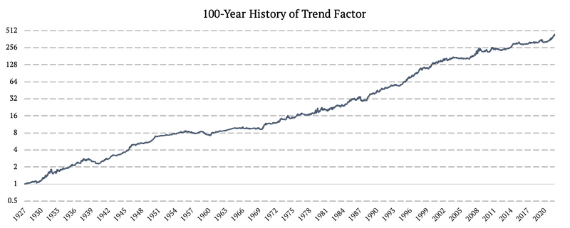
Multi-Asset Trend-Following Strategy (Trend)
Unlike the factors above, this factor is constructed as a tradable and replicable active trading strategy. The strategy trades 3 different asset classes – bonds (factor: US10Y), stocks (factor: US EQUITIES), and commodities (factor: Commodities) and applies trend-following logic. Each month we look at various trends of bonds, stocks, and commodities and go long if trend is positive or short if it’s negative. Then we weight the assets based on naïve risk parity weighting scheme.
We divided the strategy into nine sub-strategies to avoid the “timing luck bias,”. The strategy also uses various trend-following horizons All strategies are rebalanced on a monthly basis, but on different days. If you are interested in the full methodology behind the strategy, please see 100-Years of Multi-Asset Trend-Following.
Cryptocurrencies
Cryptocurrencies are the most tricky time series to model because they are the youngest major asset class. However, we can try to base our 100-years synthetic cryptocurrency time series on a research paper that compares them to high-sentiment beta stocks. Our own research confirms that cryptos are highly correlated to equities, especially during market downturns. Therefore we decided to extend cryptocurrency returns to the past by using a combination of 100% allocation to Fama & French Small Cap Low Book-to-Market quintile plus 100% allocation to Fama & French Large Cap Low Book-to-Market quintile. The resultant F&F portfolio that has a 200% allocation (mainly to growth stocks) fits the performance and volatility of cryptocurrencies relatively satisfactorily.
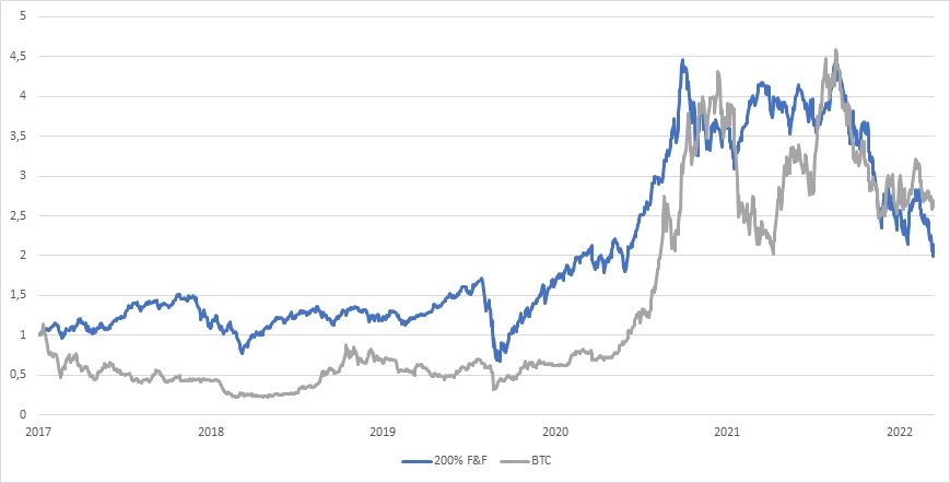
Of course, we acknowledge that our naive proxy of the cryptocurrency factor can be improved. We plan to dig deeper into this subject in the future and find an even better-fitting model which can be used as a proxy for an extended history of cryptocurrency prices… But current proxy is usable too. So to summarize:
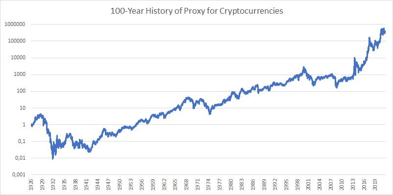
1926 – 2015: 100% Fama & French SMALL LoBM + 100% Fama & French BIG LoBM
2015 – 2022: Bitcoin Price
Multi-Factor Regression Model
After constructing 100-year history for every factor, we are ready to move to the regression model itself. The model we apply is already used in Quantpedia’s Multi-Factor Analysis tools available to all Quantpedia Pro Subscribers.
The model utilizes Akaike’s Information Criterion (AIC), which estimates the “quality“ of a model. Furthermore, the AIC accounts for the number of parameters. Therefore, the number of parameters (factors related to the given strategy) should not be too high to obtain a meaningful yet simple model with straightforward interpretations.
We employ the AIC in a model selection using the Stepwise regression with forward selection.
Suppose we have the equity curve of some strategy (independent variable). We start with a set of pre-given variables that consists of various “factors“, specifically, all factors listed in the previous section.
More generally, let’s assume that we have n factors. In the first step, we build numerous models which use only one of the factors (one factor = one model). Therefore, we are left with as many models as we have possible factors (n models). Nextly, we compute the AIC for each model, and based on the AIC, we select the best model. As the next step, we try to add another factor from the reduced set of factors that could improve our model. The algorithm builds n minus one models, computes the AIC of each model, and picks the best model.
The process where a new factor is added, based on the AIC, continues until the AIC does not improve anymore. If the AIC is not improving, it means that the model’s complexity would not outweigh the goodness of the fit of the model.
If you are interested in the full methodology behind the Multi-Factor Regression Analysis, please see our article A Robust Approach to Multi-Factor Regression Analysis.

Replicating a Balanced ETF
Now that we explained how the model works, we present an example. We replicated AOR (iShares Core Growth Allocation ETF) using our factors. From iShares: “The iShares Core Growth Allocation ETF seeks to track the investment results of an index composed of a portfolio of underlying equity and fixed income funds intended to represent a growth allocation target risk strategy.”
The AOR ETF has a history since November 2008, so the fitting is done during this period. The following figure presents the equity curves of AOR (our input portfolio) and the factor portfolio (mimicking portfolio) with the chosen factors, their weights, standard errors, and t-stat values.
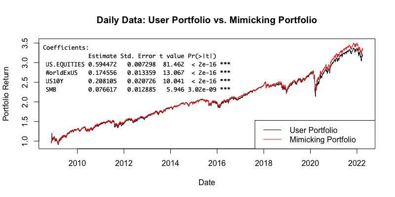
As we can see, the model chose four statistically significant factors: US EQUITIES (41.992%), WorldExUS (17.456%), US10Y (20.810%), SMB (7.662%). And these factors mimic the input portfolio (AOR US) very well – almost arriving at an identical portfolio. Thus, thanks to our model, we are able to quite precisely tell what factors drive the underlying portfolio’s returns.
Below we also present the risk/return characteristics of both portfolios.

100 years of daily ETF data
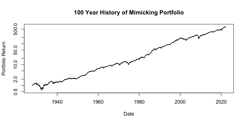
Finally, we used the calculated factor weights from our regression model and applied them to the same factors with a 100-year history. The following figure shows the equity curve of the mimicking portfolio during the past century. The chart uses log10 y-axis.
Additionally, we present the risk and return characteristics of the mimicking portfolio.
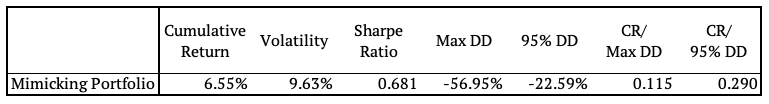
As we can see above, we were able to replicate AOR US ETF data 100 years back in history, all the way back to 1927. This gives us tremendous insights into potential development of the ETF in all sorts of bullish or bearish market scenarios. We now have a much better understanding of possible risk events and we can also make much more realistic assumptions for the performance under various scenarios and market conditions.
Conclusion
We hope this article answers multiple questions, including why being able to mimic any portfolio with factors with a 100-year history is helpful. We explained how we created such a long history for each of our 20 factors and why we chose these factors to begin with.
Subsequently, we introduced the multi-factor regression model, which picks the optimal mimicking factors of which the mimicking portfolio is made. The model utilizes Akaike’s Information Criterion (AIC) to penalize unnecessary factors, so we are left with a model that is as simple as possible with a straightforward interpretation.
We then presented AOR US ETF as a use case portfolio and compared it to the factor portfolio composed of four replicating factors, determined by Quantpedia’s model. We firstly compared the original ETF and the factor mimicking portfolio during the short history (history of AOR), and concluded that the factor replication for this ETF is almost perfect.
Lastly, and most importantly, we extended our analysis to a 100 years long history and analyzed the performance of the factor portfolio over the past century. This way we were able to quite accurately estimate the risk and return of the ETF over past 100 years.
Finally, we hope you enjoyed this article, because more will be coming soon. We are already working on the follow-up article, which will dive deeper into the 100-year history of the factor portfolio.
Author:
Daniela Hanicova, Quant Analyst, Quantpedia
Are you looking for more strategies to read about? Sign up for our newsletter or visit our Blog or Screener.
Do you want to learn more about Quantpedia Premium service? Check how Quantpedia works, our mission and Premium pricing offer.
Do you want to learn more about Quantpedia Pro service? Check its description, watch videos, review reporting capabilities and visit our pricing offer.
Are you looking for historical data or backtesting platforms? Check our list of Algo Trading Discounts.
Or follow us on:
Facebook Group, Facebook Page, Twitter, Linkedin, Medium or Youtube
Share onLinkedInTwitterFacebookRefer to a friend