There are a lot of media articles showing how "expensive" the current stock market (or some equity factor) is. However, these articles can be based on a weak statistical analysis:

Authors: Boudoukh, Israel, Richardson

Title: Long Horizon Predictability: A Cautionary Tale

Link: https://papers.ssrn.com/sol3/papers.cfm?abstract_id=3142575

Abstract:

Long-horizon return regressions have effectively small sample sizes. Using overlapping long-horizon returns provides only marginal benefit. Adjustments for overlapping observations have greatly overstated t-statistics. The evidence from regressions at multiple horizons is often misinterpreted. As a result, there is much less statistical evidence of long-horizon return predictability than implied by existing research, casting doubt over claims about forecasts based on stock market valuations and factor timing.

Notable quotations from the academic research paper:

"Pronouncements in the media about how “cheap” or “rich” the stock market or aggregate factor portfolios have become are quite common. These views also creep into the practitioner/academic finance literature.

Empirical support for these types of statements originates from seemingly “impressive” evidence of long-horizon predictability of stock returns based on valuation measures. Further, practitioners often document strong levels of statistical significance using overlapping long-horizon returns based on standard errors that they believe correct for overlapping data.

The issue is there are few independent long-horizon periods in the short samples used to study markets. Using overlapping returns in the hope of increasing the sample size offers little help. Intuitively, no matter how the data is broken down, you can’t get around the issue of short sample sizes. Therefore, findings of long-horizon predictability are illusory and reported statistical significance levels are way off. A quarter-century of statistical theory and analysis of long-horizon return regressions strongly makes this case. The bottom line is that practitioners need to be aware of these issues when performing long-horizon return forecasts and need to appropriately adjust long-horizon statistical metrics.

We show theoretically and demonstrate via simulations that there is only a marginal benefit to overlapping data for the types of return forecasting problems faced in finance. For example, in forecasting 5-year stock returns using 50 years of data, the effective number of observations, from nonoverlapping (10 periods) to monthly overlapping (600 overlapping periods), increases from 10 to just 12 observations. Statistical significance emerges only because reported standard errors (and t-statistics) are both noisy and severely biased. For example, at the 5-year stock return horizon with 50 years of data, the range of possible standard error estimates is so wide to make inference nonsensical, with the expected t-statistics effectively double their “true” value. Applying the appropriate statistics to data on long horizon stock returns and valuation ratios drastically reduces the statistical significance of these tests.

Background for Why Long-Horizon Return Regressions Are Unreliable:

To gain intuition and for illustrative purposes, the left-hand side of Figure 1 shows the scatter plot of the inverse of cyclically adjusted price earnings ratio (1/ ) and subsequent 5-year stock returns post 1968 and 10-year stock returns post 1883. Note that the number of nonoverlapping observations is 8 and 12, respectively. The point estimates of the correlations are quite large and positive, 0.26 and 0.38. However, there is very little data to back up these estimates. For example, suppose one were to take away the most outlier point in the plot; the correlations respectively become 0.04 and 0.28. Of course, this finding should not be a surprise. Under the null of no predictability, and putting aside any bias adjustment, the standard error of the correlation coefficient is 1/SQRT(T), which is 0.35 and 0.29 for 8 and 12 observations, respectively. In other words, it is quite possible the true correlation is zero or negative, especially for 5-year stock returns used in the late subsample.

In an attempt to combat this issue, practitioners will often sample long horizon stock returns more frequently using overlapping observations, believing they are increasing their sample sizes significantly. Consistent with this observation, the overlapping scatter plots on the right-hand side of Figure 1 are instark contrast to those on the left-hand side and appear to show overwhelming evidence of a strong positive relation.

For example, in referring to 1/CAPE’s ability to forecast 10-year returns relative to his previous work, Shiller writes in chapter 11 of the latest edition of his book, Irrational Exuberance, “We now have data from 17 more years, 1987 through 2003 (end-points 1997 through 2013), and so 17 new points have been added to the 106 (from 1883)".  As such, in describing this estimated positive relation between 1/CAPE and future long-term returns, Shiller (2015) writes “…the swarm of points in the scatter shows a definite tilt.”

This is fallacy.

In Shiller’s above example, because 1/CAPE (measured as a 10-year moving average of earnings) is highly persistent, only 2, not 17, nonoverlapping observations have been truly added. To see this, note that standing in January 2003 versus in January 2004, looking ahead 10 years in both cases, the future 10-year returns have 9-years in common. So even if stock returns are serially independent through time, the 10-year return in adjacent years will be 0.90 correlated by construction. Moreover, 1/CAPE itself has barely changed due to its 10-year moving average of earnings and fundamental persistence of stock prices during the period between January 2003 and January 2004. It is these facts that create, by construction, Shiller’s “swarm” effect, visible in the figures. In reality, there is just a smattering of independent data points, 12 to be precise.”"

Are you looking for more strategies to read about? Check http://quantpedia.com/Screener

Do you want to see performance of trading systems we described? Check http://quantpedia.com/Chart/Performance

Do you want to know more about us? Check http://quantpedia.com/Home/About

Follow us on:

Facebook: https://www.facebook.com/quantpedia/

Twitter: https://twitter.com/quantpedia

Nice academic paper uses Metcalfe’s law to estimate Bitcoin's fundamental value. A really recommended read … :

Authors: Wheatley, Sornette, Huber, Reppen, Gantner

Title: Are Bitcoin Bubbles Predictable? Combining a Generalized Metcalfe's Law and the LPPLS Model

Link: https://papers.ssrn.com/sol3/papers.cfm?abstract_id=3141050

Abstract:

We develop a strong diagnostic for bubbles and crashes in bitcoin, by analyzing the coincidence (and its absence) of fundamental and technical indicators. Using a generalized Metcalfe’s law based on network properties, a fundamental value is quantified and shown to be heavily exceeded, on at least four occasions, by bubbles that grow and burst. In these bubbles, we detect a universal super-exponential unsustainable growth. We model this universal pattern with the Log-Periodic Power Law Singularity (LPPLS) model, which parsimoniously captures diverse positive feedback phenomena, such as herding and imitation. The LPPLS model is shown to provide an ex-ante warning of market instabilities, quantifying a high crash hazard and probabilistic bracket of the crash time consistent with the actual corrections; although, as always, the precise time and trigger (which straw breaks the camel’s back) being exogenous and unpredictable. Looking forward, our analysis identifies a substantial but not unprecedented overvaluation in the price of bitcoin, suggesting many months of volatile sideways bitcoin prices ahead (from the time of writing, March 2018).

Notable quotations from the academic research paper:

"The explosive growth of bitcoin intensified debates about the cryptocurrency’s intrinsic or fundamental value. While many pundits have claimed that bitcoin is a scam and its value will eventually fall to zero, others believe that further enormous growth and adoption await, often comparing to the market capitalization of monetary assets, or stores of value. By comparing bitcoin to gold, an analogy that is based on the digital scarcity that is built into the bitcoin protocol, some markets analysts predicted bitcoin prices as a high as 10 million per bitcoin.

There is an emerging academic literature on cryptocurrency valuations and their growth mechanisms. Many of these studies attribute some technical feature of the bitcoin protocol, such as the “proof-of-work” system on which the bitcoin cryptocurrency is based, as a source of value. However, as has been proposed by former Wall Street analyst Tom Lee, an early academic proposal, by now widely discussed within cryptocurrency communities, is that an alternative valuation of bitcoin can be based on its network of users. In the 1980s, Metcalfe proposed that the value of a network is proportional to the square of the number of nodes. This may also be called the network effect, and has been found to hold for many networked systems. If Metcalfe’s law holds here, fundamental valuation of bitcoin may in fact be far easier than valuation of equities—which relies on various multiples, such as price-to-earnings, price-to-book, or price-to-cash-flow ratios—and will therefore admit an indication of bubbles.

Here, we combine—as a fundamental measure—a generalized Metcalfe’s law and—as a technical measure—the LPPLS model, in order to diagnose bubbles in bitcoin. When both measures coincide, this provides a convincing indication of a bubble and impending correction. If, in hindsight, such signals are followed by a correction similar to that suggested, they provide compelling evidence that a bubble and crash did indeed take place.

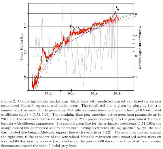
Given the number of active users, and calibrations of the generalized Metcalfe’s law, which maps to market cap, we can now compare the predicted market cap with the true one, as in Figure 2. Also, using smoothed active users, the local endogeneities—where price drives active users—are assumed to be averaged out. The OLS estimated regression, by definition, fits the conditional mean, as is apparent in Figure 2. Therefore, if bitcoin has evolved based on fundamental user growth with transient overvaluations on top, then the OLS estimate will give an estimate in-between and thus above the fundamental value. For this reason, support lines are also given, and—although their parameters are chosen visually—they may give a sounder indication of fundamental value. In any case, the predicted values for the market cap indicate a current over-valuation of at least four times. In particular, the OLS fit with parameters (1.51,1.69), the support line with (0,1.75), and the Metcalfe support line (-3,2) suggest current values around 44, 22, and 33 billion USD, respectively, in contrast to the actual current market cap of 170 billion USD. Further, assuming continued user growth in line with the regression of active users starting in 2012, the end of 2018 Metcalfe predictions for the market cap are 77, 39, and 64 billion USD respectively, which is still less than half of the current market cap. These results are found to be robust with regards to the chosen fitting window.

"

Are you looking for more strategies to read about? Check http://quantpedia.com/Screener

Do you want to see performance of trading systems we described? Check http://quantpedia.com/Chart/Performance

Do you want to know more about us? Check http://quantpedia.com/Home/About

Follow us on:

Facebook: https://www.facebook.com/quantpedia/

Twitter: https://twitter.com/quantpedia

A recent academic research looks at effects of algorithmic trading during turbulent times:

Authors: Breedon, Chen, Ranaldo, Vause

Title: Judgement Day: Algorithmic Trading Around the Swiss Franc Cap Removal

Link: https://papers.ssrn.com/sol3/papers.cfm?abstract_id=3126136

Abstract:

A key issue raised by the rapid growth of computerised algorithmic trading is how it responds in extreme situations. Using data on foreign exchange orders and transactions that includes identification of algorithmic trading, we find that this type of trading contributed to the deterioration of market quality following the removal of the cap on the Swiss franc on 15 January 2015, which was an event that came as a complete surprise to market participants. In particular, we find that algorithmic traders withdrew liquidity and generated uninformative volatility in Swiss franc currency pairs, while human traders did the opposite. However, we find no evidence that algorithmic trading propagated these adverse effects on market quality to other currency pairs.

Notable quotations from the academic research paper:

"We analyse the role of AT in foreign exchange (FX) markets in a period containing the 15 January 2015 announcement by the Swiss National Bank that it had discontinued its policy of capping the value of the Swiss franc against the euro. This ‘Swiss franc event’ represents a natural experiment as one of the largest shocks to the FX market in recent years and probably the most significant ‘black swan’ event in the period in which AT has been a prominent force in FX markets. In particular, we study the contribution of AT and human traders to two important dimensions of market quality, namely liquidity and price efficiency. Our analysis is based on a unique dataset with a detailed identification of AT obtained from EBS Market, which is the leading platform for electronic spot FX trading in many of the major currencies.

A detailed understanding of AT in distressed situations is important for at least two reasons. First, a better comprehension of whether AT is beneficial or detrimental for market quality in extreme situations would help inform the ongoing reform of trading venues. Second, the resilience of an exchange system depends on the behaviour of different types of market participant and their reciprocal influence on each other. For instance, a tendency of AT to offer liquidity in calm markets and withdraw it in distressed situations could lead less sophisticated agents to become reliant on high levels of market liquidity only to find it in short supply when they most needed it. If these adverse consequences of AT were predominant or not offset by other traders, then AT could represent a systemic threat to the whole trading system. To shed light on this key issue for financial stability, we analyse whether human traders and AT substitute for or complement each other in supplying and consuming liquidity.

We proceed in three steps. First, we describe the EBS Market platform and our sample of data from it. Second, we perform an in-depth analysis of market liquidity and price movements by decomposing order flow, effective spreads and intraday volatility by type of trader. This enables us to highlight the contribution of AT and human traders to liquidity provision and consumption, transaction costs and realised volatility. Third, we study the contribution to efficient pricing of AT and human traders.

Our study delivers two important findings. First, in reaction to the Swiss franc event, we find that AT tended to consume liquidity and reinforce the price disruption. Opposite and offsetting patterns apply for human traders, who supported market quality by providing liquidity and aiding price discovery. Second, we find that this market quality degradation coming from AT was concentrated in the shocked FX rate (EUR/CHF) and, to a lesser extent, USD/CHF. Non-CHF currency pairs (USD/JPY, EUR/JPY and EUR/USD in our sample) were essentially unaffected.3 This suggests that AT models were somewhat compartmentalised, which, along with human trading, helped to sustain market quality beyond the CHF currency pairs.

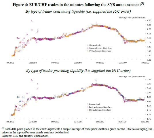
Figure 4 shows the prices at which different types of trader exchanged euros for Swiss francs in the 30 minutes following the SNB announcement depending on whether their trades were consuming liquidity (top panel) or providing it (bottom panel). Trades that consume liquidity result from IOC orders, while those that provide it result from GTC orders. The top panel shows that bank AIs consumed liquidity at extreme prices (prices significantly different to those of immediately preceding trades) on a number of occasions, notably between 9.31 and 9.36. Thus, over 75% of the cumulative appreciation of the franc in the 20 minutes to 9.50 was attributable to bank AIs, which accounted for 61% of the volume of liquidity-consuming trades. Indeed, we show below that bank AIs accounted for an even larger share of the realised variance of the EUR/CHF rate at this time. The lower panel shows that bank AIs also provided liquidity for some of the extreme-price trades. That bank AIs both consumed and provided liquidity at extreme prices may reflect the diverse set of traders from whom these trades may originate. This includes not only the different banks but also their various clients. In addition, a roughly equal number of extreme-price trades were accommodated by human traders. Indeed, human traders accounted for a significantly higher share of liquidity-providing trades (50%) than they did for liquidity-consuming trades (19%) during the 20 minutes to 9.50 when the Swiss franc appreciated sharply.

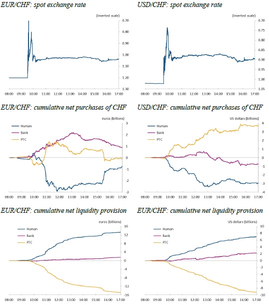
Figure 5 gives an overview of the reaction of both the EUR/CHF and USD/CHF markets to the SNB announcement over the whole trading day of 15 January 2015. The first row shows that the Swiss franc appreciated extremely sharply against both ‘base’ currencies in the first 20 minutes following the announcement, but that sizeable portions of these gains were reversed in the subsequent hour. After that the two spot rates were much more stable, with the Swiss franc worth about 10% more than at the start of the day. The second row shows that algorithmic traders were net purchasers of Swiss francs over the day, particular bank AIs against the euro and PTC AIs against the US dollar, while human traders were net purchasers of the base currencies. Thus, computers traded ‘with the wind’, buying the franc as it appreciated, while humans ‘leaned against the wind’. Note, however, that human traders did not make net purchases of the base currencies in the key 20-minute period immediately after the announcement. Finally, the third row shows that human traders were consistently net suppliers of liquidity over the day, while PTC AI trades consumed it. However, as we shall see below, net liquidity consumption by PTC AIs is not unusual in these two currency-pairs.

"

Are you looking for more strategies to read about? Check http://quantpedia.com/Screener

Do you want to see performance of trading systems we described? Check http://quantpedia.com/Chart/Performance

Do you want to know more about us? Check http://quantpedia.com/Home/About

Follow us on:

Facebook: https://www.facebook.com/quantpedia/

Twitter: https://twitter.com/quantpedia

A new financial research paper related to:

#13 – Short Term Reversal in Stocks

Authors: Drechsler, Moreira, Savov

Title: Liquidity Creation As Volatility Risk

Link: https://papers.ssrn.com/sol3/papers.cfm?abstract_id=3133291

Abstract:

We show, both theoretically and empirically, that liquidity creation induces negative exposure to volatility risk. Intuitively, liquidity creation involves taking positions that can be exploited by privately informed investors. These investors' ability to predict future price changes makes their payoff resemble a straddle (a combination of a call and a put). By taking the other side, liquidity providers are implicitly short a straddle, suffering losses when volatility spikes. Empirically, we show that short-term reversal strategies, which mimic liquidity creation by buying stocks that go down and selling stocks that go up, have a large negative exposure to volatility shocks. This exposure, together with the large premium investors demand for bearing volatility risk, explains why liquidity creation earns a premium, why this premium is strongly increasing in volatility, and why times of high volatility like the 2008 financial crisis trigger a contraction in liquidity. Taken together, these results provide a new, asset-pricing view of the risks and rewards to financial intermediation.

Notable quotations from the academic research paper:

"We show, both theoretically and empirically, that liquidity creation—making assets cheaper to trade than they otherwise would be—induces exposure to volatility risk. Given the very large premium investors pay to avoid volatility risk, this explains why liquidity creation earns a premium, why this premium is strongly increasing in volatility, and why times of high volatility like the 2008 financial crisis trigger a contraction in liquidity.

Why does liquidity creation induce exposure to volatility risk? To create liquidity for some investors in an asset, a liquidity provider takes positions that can be exploited by other, privately informed investors. These investors buy the asset if they think it will rise in value and sell it if they think it will fall. Their ex post payoff therefore resembles a straddle (a combination of a call and a put option). Like any straddle, this payoff is high if volatility rises and low if it falls. By taking the other side, the liquidity provider is implicitly short the straddle, earning a low payoff if volatility rises and a high one if it falls. In other words, the liquidity provider is exposed to volatility risk.

The relation between liquidity creation and volatility risk is fundamental; it arises directly from the presence of asymmetric information. As a result, it applies widely across a variety of market structures. For instance, one way financial institutions create liquidity is by issuing relatively safe securities against risky assets. In doing so, they are betting against private information possessed by those who originate the assets or in some other way take a position against them (e.g. through derivatives). Consequently, when volatility spikes and this private information becomes more valuable, financial institutions suffer losses, as they did during the 2008 financial crisis.

Financial institutions and other investors also create liquidity by trading in secondary markets such as those for stocks and bonds. We present a model to formalize how this type of liquidity creation induces volatility risk and how this risk drives the liquidity premium. We also use the model to motivate our empirical analysis.

We test the predictions of our model using U.S. stock return data from 2001 to 2016 (covering the period after “decimalization,” when liquidity provision became competitive). Each day, we sort stocks into deciles based on their return (normalized by its rolling standard deviation) and quintiles based on their size (small stocks are known to be much less liquid). Within each size quintile, we construct longshort portfolios that buy stocks in the low return deciles and sell stocks in the high return deciles. These are known as short-term reversal portfolios in the literature. In our model, a large return reflects high order flow and hence high liquidity demand. The reversal portfolio therefore mimics the position of the liquidity provider, hence, we can use it to analyze the returns to liquidity creation.

Consistent with the model, and with the prior literature, our reversal portfolios earn substantial returns that cannot be explained by exposure to market risk. Among large stocks, which account for the bulk of the market by value, the reversal strategy across the lowest and highest return deciles has an average return of 27 bps over a five day holding period, or about 13.5% per year. The annual Sharpe ratio is 0.6.

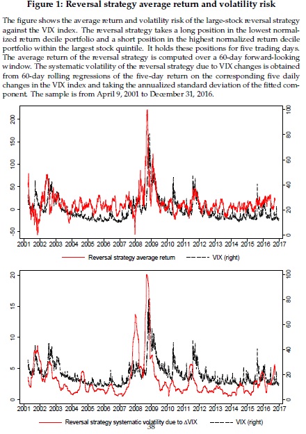
Figure 1 plots the return of the large-stock reversal strategy averaged over a 60-day forward-looking window against the level of VIX, a risk-neutral measure of the expected volatility of the S&P 500 over the next 30 days. The figure shows that the reversal return is strongly positively related to VIX (the raw correlation is 46%). In a regression, we find that a one-point higher VIX leads to a 5.37 bps higher reversal return over the next five days, which is large relative to the average return of the strategy. The R2 of this regression is 2.18%, which is very high for daily data. These findings confirm the main result of Nagel that VIX predicts reversal returns. They are also a prediction of our model. A high level of VIX is associated not only with high expected volatility but also with high volatility of volatility (and high aversion to volatility risk). In our model this makes liquidity creation riskier and raises the price of liquidity.

The bottom panel of Figure 1 tests this mechanism by plotting a measure of the volatility risk of the reversal strategy. We compute it by running 60-day rolling window regressions of the five-day large-stock reversal return on the daily VIX changes during the holding period. The figure plots the annualized standard deviation of the fitted value from this regression, which captures the systematic volatility of the reversal strategy due to VIX changes, i.e. its volatility risk. The figure shows that the volatility risk of the reversal strategy is substantial and that it covaries strongly with the level of VIX (the raw correlation is 58%). This confirms the prediction that when VIX is high the reversal strategy is exposed to more volatility risk, which is consistent with its higher premium.

"

Are you looking for more strategies to read about? Check http://quantpedia.com/Screener

Do you want to see performance of trading systems we described? Check http://quantpedia.com/Chart/Performance

Do you want to know more about us? Check http://quantpedia.com/Home/About

A new financial research paper related to:

#12 – Pairs Trading with Stocks

Authors: Farago,Hjalmarsson

Title: Stock Price Co-Movement and the Foundations of Pairs Trading

Link: https://papers.ssrn.com/sol3/papers.cfm?abstract_id=3114058

Abstract:

We study the theoretical implications of cointegrated stock prices on the profitability of pairs trading strategies. If stock returns are fairly weakly correlated across time, cointegration implies very high Sharpe ratios. To the extent that the theoretical Sharpe ratios are "too large," this suggests that either (i) cointegration does not exist pairwise among stocks, and pairs trading profits are a result of a weaker or less stable dependency structure among stock pairs, or (ii) the serial correlation in stock returns stretches over considerably longer horizons than is usually assumed. Empirically, there is little evidence of cointegration, favoring the first explanation.

Notable quotations from the academic research paper:

"The purpose of the current paper is to evaluate whether cointegration among stockprices is indeed a realistic assumption upon which to justify pairs trading. In particular, we derive the expected returns and Sharpe ratios of a simple pairs trading strategy, under the assumption of pairwise cointegrated stock prices, allowing for a flexible specification of the stochastic process that governs the individual asset prices. Our analysis shows that, under the typical assumption that stock returns only have weak and fairly short-lived serial correlations, cointegration of asset prices would result in extremely profitable pairs trading strategies. In a cointegrated setting, a typical pairs trade might easily have an annualized Sharpe ratio greater than ten, for a single pair, ignoring any diversification benefits of trading many pairs simultaneously. Cointegration of stock prices therefore appears to deliver pairs trading profits that are "too good to be true."

The existence of cointegration essentially implies that the deviations between two nonstationary series is stationary. The speed at which the two series converge back towards each other after a given deviation depends on the short-run, or transient, dynamics in the two processes. If there are relatively long-lived transient shocks to the series, the two processes might diverge from each other over long periods, although cointegration ensures that they eventually converge. If the transient dynamics are short-lived, the two series must converge very quickly, once they deviate from each other. In the latter case, most shocks to the series are of a permanent nature and therefore subject to the cointegrating restriction, which essentially says that any permanent shock must affect the two series in an identical manner.

To put cointegration in more economic terms, consider a simple example of two different car manufacturers. If both of their stock prices are driven solely by a single common factor, e.g., the total (expected long-run) demand for cars, then the two stock prices could easily be cointegrated. However, it is more likely that the stock prices depend on firm-specific demands, which contain not only a common component but also idiosyncratic components. In this case, the idiosyncratic components of demands will cause deviations between the two stock prices, and price cointegration would require that the idiosyncratic demands only cause temporary changes in the stock prices. That is, cointegration imposes the strong restriction that any idiosyncratic effects must be of a transient nature, such that they do not cause a permanent deviation between the stock prices of different firms.

In the stock price setting considered here, most price shocks are usually thought to be of a permanent nature. For instance, under the classical random walk hypothesis, all price shocks are permanent. Although current empirical knowledge suggests that there are some transient dynamics in asset prices, these are usually thought to be small and short lived. In this case, if two stock prices are cointegrated, there is very little scope for them to deviate from each other over long stretches of time. Thus, when a transient shock causes the two series to deviate, they will very quickly converge back to each other. Such quick convergence is, of course, a perfect setting for pairs trading, and gives rise to the outsized Sharpe ratios implied by the theoretical analysis.

The theoretical analysis thus predicts that cointegration among stock prices leads to statistical arbitrage opportunities that are simply too large to be consistent with the notion that markets are relatively efficient, and excess profits reasonably hard to achieve. Or, alternatively, the serial correlation in stock returns must be considerably longer-lived than is usually assumed, with serial dependencies stretching at least upwards of six months. However, such long-lived transient dynamics imply a rather slow convergence of prices in pairs trades, at odds with the empirical evidence from pairs trading studies.

In the second part of the paper, we evaluate to what extent there is any support in the data for the predictions of the cointegrated model.

The theoretical and empirical analysis together strongly suggest that cointegration is not a likely explanation for the profitability of pairs trading strategies using ordinary pairs of stocks. Pairs trading is based on the idea of stock prices co-moving with each other, and that deviations from this co-movement will be adjusted and reverted, such that prices eventually converge after deviating. Profitability of such strategies is consistent with cointegration, but cointegration is not a necessary condition for pairs trading to work. Instead, it is quite likely that pairs trading profits arise because over shorter time spans, asset prices on occasion move together. This could, for instance, be due to fundamental reasons, such as a common and dominant shock affecting all stocks in a given industry."

Are you looking for more strategies to read about? Check http://quantpedia.com/Screener

Do you want to see performance of trading systems we described? Check http://quantpedia.com/Chart/Performance

Do you want to know more about us? Check http://quantpedia.com/Home/About

A new financial research paper related to:

#5 – FX Carry Trade

Authors: Orlov

Title: Solvency Risk Premia and the Carry Trades

Link: https://papers.ssrn.com/sol3/papers.cfm?abstract_id=3116031

Abstract:

This paper shows that currency carry trades can be rationalized by the time-varying risk premia originating from the sovereign solvency risk. We find that solvency risk is a key determinant of risk premia in the cross section of carry trade returns, as its covariance with returns captures a substantial part of the cross-sectional variation of carry trade returns. Importantly, low interest rate currencies serve as insurance against solvency risk, while high interest rate currencies expose investors to more risk. The results are not attenuated by existing risks and pass a broad range of various robustness checks.

Notable quotations from the academic research paper:

"Overall, the cumulative evidence points to time-varying risk premia as the pervasive source of the carry trade returns and to the forward premium puzzle not being without costs. Nonetheless, the identification of an appropriate risk premia that explains the carry trade profitability remains an ongoing debate. This paper provides new evidence in favor of sovereign solvency being a potential source of risk in currency market.

This paper contributes to current debate by revealing a new economic-based time-varying risk premia in the currency market that depends upon a country’s solvency. We argue that the financial capacity of the economy, captured by the solvency measures, incites the differences in average carry trade excess returns. In other words, the profitability of currency carry trades can be rationalized by the time-varying risk premia that originate from the sovereign solvency risk. Consistently, we find that high interest rate currencies demand a higher risk premium, as they deliver low carry trade returns at times of high solvency risk, therefore exposing investors to more risk, whereas low interest currencies are a hedge against the solvency risk.

In this paper we assume risk premium is a function of financial solvency of the economy, defined by either a ratio of foreign debt to economy’s earning ability (henceforth, the solvency measure), or a ratio of balance of the current account to the estimated aggregate of total exports of goods and services, or aggregated financial solvency index. Risk premium is then represented by an increasing convex function of one of these measures. In the most of our analysis, we consider external debt service capacity measured by the gross foreign debt-to-output ratio as a measure of solvency of the country.

We perform portfolio sorts on forward discounts and the solvency measure, identify risk factor as the returns on zero-cost long-short strategy between the last and first solvency-sorted portfolios and label it IMS, for indebted-minus-solvent economies. The IMS factor explains the substantial part of the cross-sectional variation in carry trade portfolios, exhibiting monotonically increasing factor loadings and significant prices of risk, consistent with risk premia explanation. Moreover, the factor is empirically powerful in various model specifications and sample splits, prices different test assets, stands out horse races with other currency-specific risk factors, robust against an alternative funding currency (the Japanese Yen) and alternative solvency measure specifications, and passes several other robustness checks. Taken collectively pointing to the solvency risk factor being an effective tool for pricing the cross-section of carry returns."

Are you looking for more strategies to read about? Check http://quantpedia.com/Screener

Do you want to see performance of trading systems we described? Check http://quantpedia.com/Chart/Performance

Do you want to know more about us? Check http://quantpedia.com/Home/About