Our favorite research paper about the performance of long-only investment strategies in commodities:

Authors: Erb, Harvey

Title: Conquering Misperceptions about Commodity Futures Investing

Link: https://papers.ssrn.com/sol3/papers.cfm?abstract_id=2645444

Abstract:

Long-only commodity futures returns have been very disappointing over the last decade, leading some to wonder if it was a mistake to invest in commodities. The poor performance is the result of poor “income returns” and not of falling commodity prices. This observation may be surprising for many commodity investors who were not aware, who misperceived, they were making a bet on income returns, a return building block similar to a stock’s dividend yield or a bond’s yield. For investors seeking an inflation hedge, it may be surprising that the historical linkage of commodity returns with inflation seems to be the result of a connection between commodity income returns and inflation, not, as commonly misperceived, commodity price returns and inflation. It may be surprising that the value of commodity investments is smaller than the market capitalization of Facebook, a potentially striking misperception for investors seeking a portfolio diversifier with abundant capacity. There has been no change in the way that price returns and income returns drive the total returns of stocks, bond and commodities. What has changed is that maybe a good number of commodity investors now realize that they were operating outside of their “circle of competence” and did not have a sense of what future price and income returns could be and would be.

Notable quotations from the academic research paper:

"The last ten years have been challenging for many long‐only commodity futures investors and given many a reason to question whether a ‘bad’ investment strategy drove a bad outcome or a ‘good’ strategy experienced an unlucky outcome. The total return of the S&P GSCI commodity index was ‐4.6% per year, much lower than the +7.4% return for the S&P 500 stock index and the +4.5% return for the Barclays U.S. Aggregate bond index. The key driver of the poor S&P GSCI performance has been a ‐8.0% income return. The commodity income return is the sum of a collateral return (in this case the three‐month Treasury bill) and a roll return (the cost, or benefit, of staying invested in futures contracts over time).

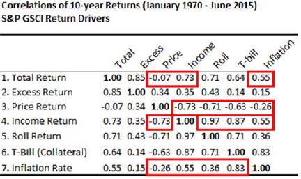
What has driven commodity portfolio returns? Focusing on the investable commodity index with the longest performance history, the S&P GSCI, Exhibit 3 shows correlations for rolling 10‐year returns for the drivers of the S&P GSCI. What seemingly drove commodity total returns? Interestingly, the first row shows that, historically, there has been little correlation between total return and price return (‐0.07), a high correlation between total return and income return (0.73) and a positive correlation between total return and inflation (0.55). What drove commodity price returns? The third row shows that historically price returns were negatively correlated with income returns (‐0.73), with roll returns (‐0.71), with collateral returns (‐0.63) and with inflation (‐0.26). What drove income returns? The fourth row shows that historically income returns were positively correlated with roll returns (0.97), with collateral returns (0.87) and with inflation (0.55). Finally, which commodity return components were correlated with inflation? The seventh row shows that price returns were negatively correlated with inflation (‐0.26), positively correlated with income returns (0.55), positively correlated with roll returns (0.36) and positively correlated with collateral returns (0.83). In a broad sense, Exhibit 3 suggests:

1) a weak link between commodity price returns and commodity total returns,

2) a negative link between inflation and commodity price returns,

3) a positive link between commodity income returns and commodity total returns,

4) a positive link between inflation and commodity income returns and

5) a negative relationship between income returns and price returns.

There are at least two opposing views to explain the decline in income and roll returns. The first view offered by Bhardwaj, Gorton and Rouwenhorst (2015) is that there is in fact no difference between pre‐2004 commodity performance and post‐2004 commodity performance. Their view is illustrated by looking at the performance of a hypothetical, equally‐weighted paper portfolio created by Gorton and Rouwenhorst (2006). This paper portfolio embeds a common smart beta strategy, rebalancing an equally weighted portfolio. Working with an intuition that commodity futures markets are risk transfer insurance markets for commodity hedgers, Bhardwaj, Gorton and Rouwenhorst also find no evidence that an influx of long‐only financial commodity investors over the last decade has impacted the historical or prospective returns of their hypothetical paper portfolio. Summing up the impact of the last decade, they find “the risk premium has been comparable to its long‐term historical average”.

Norrish (2015) argues that Gorton and Rouwenhorst’s hypothetical paper portfolio “is not a viable option for most investors”, and reflects an alternative view that over the last decade an influx of long‐only financial investors significantly lowered returns for actual and tradable long‐only commodity indices. Echoing the view that commodity futures markets can be viewed as price insurance markets, Norrish’s view is that there has been too much long‐only insurance capital chasing too few insurance opportunities. If too much insurance‐inspired capital has lowered returns then perhaps a contraction in insurance inspired capital might increase returns."

Are you looking for more strategies to read about? Check http://quantpedia.com/Screener

Do you want to see performance of trading systems we described? Check http://quantpedia.com/Chart/Performance

Do you want to know more about us? Check http://quantpedia.com/Home/About

An interesting academic paper about the intristic value of Gold:

Authors: Harris, Shen

Title: The Intrinsic Value of Gold: An Exchange Rate-Free Price Index

Link: https://papers.ssrn.com/sol3/papers.cfm?abstract_id=2926454

Abstract:

In this paper, we propose a gold price index that enables market participants to separate the change in the ‘intrinsic’ value of gold from changes in global exchange rates. The index is a geometrically weighted average of the price of gold denominated in different currencies, with weights that are proportional to the market power of each country in the global gold market, where market power is defined as the impact that a change in a country’s exchange rate has on the price of gold expressed in other currencies. We use principal components analysis to reduce the set of global exchange rates to four currency ‘blocs’ representing the U.S. dollar, the euro, the commodity currencies and the Asian currencies. We estimate the weight of each currency bloc in the index in an error correction framework using a broad set of variables to control for the unobserved intrinsic value. We show that the resulting index is less volatile than the USD price of gold and, in contrast with the USD price of gold, has a strong negative relationship with global equities and a strong positive relationship with the VIX index, both of which underline the role of gold as a safe haven asset.

Notable quotations from the academic research paper:

"The market for gold is one of the largest and most liquid in the world, surpassed only by the major currency pairs in terms of daily turnover. The price of gold, like that of many commodities, is conventionally quoted in USD. However, gold is not exclusively a US asset and so the return from an investment in gold, when calculated using the quoted USD price, conflates the change in the value of gold with the change in the value of the USD. In this paper, we develop a gold price index, which when used to compute returns, reflects changes in the intrinsic value of gold independently of concurrent changes in global exchange rates.

Various index-based approaches go some way towards removing the exchange rate component of the gold price, they do not properly reflect the intrinsic value of gold because they use arbitrarily defined weights that do not represent the actual impact that changes in individual exchange rates have on the quoted gold price.

The gold price index that we develop can be thought of as a geometric weighted average of the normalized real (i.e. inflation-adjusted) price of gold in different currencies. The weight of each currency is proportional to that country’s market power in the global gold market, as reflected in the impact that a change in the country’s real exchange rate has on the real price of gold quoted in other currencies. We cast the relationship between the price of gold, exchange rates and a broad set of fundamental variables in a cointegration framework, in which we simultaneously model both the long run relationship between the price of gold and its determinants, and its short run dynamics. We use weekly data from 3 January 1995 to 26 October 2015 for 23 exchange rates against the GBP. In view of the very high correlations between many individual exchange rates, we use principal components analysis to extract the significant underlying exchange rate factors.

Over the full sample, we find that there are four ‘significant’ principal components in real exchange rates, which are shown to represent the USD currency bloc, the commodity currency block, the EUR currency block, and the Asian currency bloc, respectively. The cointegration framework allows us to distinguish between the long run and short run elasticities of the price of gold with respect to exchange rates. In particular, the long run elasticity with respect to an exchange rate (or an exchange rate bloc) partially reflects structural changes and, in particular, the impact that a change in the exchange rate has on fundamentals through, for example, changes in production capacity or demand. In contrast, the short run elasticity reflects the change in the gold price arising directly from changes in the exchange rate, i.e. changes in the price of gold that simply reflect ‘translation’ effects. It is these short run elasticities that are relevant for the construction of the gold price index.

We therefore first estimate the long run relationship between the real price of gold, real exchange rates and proxies for the non-exchange rate related fundamentals, including global equity and bond prices, the oil price and the level of the VIX index of implied volatility, and show that these variables are strongly cointegrated. The gold price has a negative long run relation with global equity prices and a positive long run relation with global bond prices, the price of oil and the VIX index. Gold has a positive long run relationship with the USD bloc, the EUR bloc and the commodity currency bloc, but a somewhat weaker relationship with the Asian currency bloc.

We then estimate the short run dynamics of the change in the gold price as a function of (1) changes in exchange rates, (2) changes in fundamentals and (3) the lagged error correction term that captures the deviation from long run equilibrium. The short run elasticities from this regression are then used as weights in the gold price index. Using the full sample to estimate the model, we show that the (normalized) weights on the USD bloc, the commodity bloc and the EUR bloc are about 21%, 48% and 31%, respectively, reflecting the relative importance of these currency blocks for production, consumption and investment in the global gold market. The weight on the Asian currency bloc is not significantly different from zero. We convert the real gold price index into a nominal USD gold price index to enable a comparison with the USD price of gold. We show that the nominal gold price index is less volatile than the USD gold price and, in contrast with the USD gold price, has a strong negative relationship with global equities and a strong positive relationship with the VIX index, both of which underline the role of gold as a safe haven asset."

Are you looking for more strategies to read about? Check http://quantpedia.com/Screener

Do you want to see performance of trading systems we described? Check http://quantpedia.com/Chart/Performance

Do you want to know more about us? Check http://quantpedia.com/Home/About

A recent paper takes a look on Time-Series (TS) vs. Cross-Sectional (CS) version of momentum strategy. Analysis is made on equities but, in our opinion, has implication also on TS vs. CS momentum strategies on futures.

Authors: Cheema, Nartea, Man

Title: Cross-Sectional and Time-Series Momentum Returns and Market States

Link: https://papers.ssrn.com/sol3/papers.cfm?abstract_id=2931620

Abstract:

Recent evidence on momentum returns shows that the time-series (TS) strategy outperforms the cross-sectional (CS) strategy. We present new evidence that this happens only when the market continues in the same state, UP or DOWN. In fact, we find that the TS strategy underperforms the CS strategy when the market transitions to a different state. Our results show that the difference in momentum returns between TS and CS strategies is related to both the net long and net short positions of the TS strategy.

Notable quotations from the academic research paper:

"The recent evidence on momentum returns suggests that the time-series (TS) strategy proposed by Moskowitz, Ooi and Pedersen (2012) outperforms the cross-sectional (CS) strategy of Jegadeesh and Titman (1993) because of its stock selection abilities. However, Goyal and Jegadeesh (2015) show that the TS strategy outperforms the CS because of the compensation of its net long position instead of its stock selection abilities. They argue that TS is a combination of a zero-net investment strategy and a net long investment in the risky assets, whereas CS is an entirely zero-cost strategy. Therefore, the compensation of the net long investment in risky assets enhances the performance of the TS strategy which not only earns the risk premium relative to the CS strategy but also benefits from market timing because there are more up than down markets.

In this paper, we empirically examine whether the TS strategy outperforms the CS strategy because of its net long position by conditioning momentum returns on market states. We define market states based on lagged 12-month (t-11) and subsequent month (t+1) Centre for Research in Security Prices (CRSP) value-weighted market returns. A market state is identified as UP/UP (DN/DN) when the lagged, and subsequent market returns are both positive (negative). We classify the market state as UP/DN (DN/UP) if the lagged 12-month returns are positive (negative) and the subsequent market returns are negative (positive).

To the extent that momentum returns of the TS strategy exceed the CS strategy because of its net long position as suggested by Goyal and Jegadeesh (2015), then TS momentum returns would be relatively higher in UP/UP market because the net long position would time the subsequent UP market. However, if TS momentum returns exceed the CS because of its active position whether net long or net short, then we should expect relatively higher TS momentum return in market continuations whether UP/UP or DN/DN because the net long (net short) position times the subsequent UP (DN) market. Furthermore, we expect that the TS strategy would underperform the CS strategy in market transitions (UP/DN or DN/UP) because the net long (short) position of the TS strategy negatively times the subsequent DN (UP) market.

Consistent with our expectations, we find that the TS strategy outperforms (underperforms) the CS strategy only in market continuations (transitions). We find that the net long/short position times the market in market continuations which enhances TS momentum returns. However, in market transitions, the net long/short position exhibit negative autocorrelation with the subsequent market returns which results into larger losses for the TS strategy."

Are you looking for more strategies to read about? Check http://quantpedia.com/Screener

Do you want to see performance of trading systems we described? Check http://quantpedia.com/Chart/Performance

Do you want to know more about us? Check http://quantpedia.com/Home/About

A recent paper gives a summary of theoretical explanations of asset price properties (based on neurology) and reasons for trendfollowing strategies. Related to all trend-based strategies, mainly to:

#1 – Asset Class Trend Following
#144 – Trendfollowing Effect in Stocks

Authors: Bouchaud, Challet

Title: Why have asset price properties changed so little in 200 years

Link: https://arxiv.org/pdf/1605.00634.pdf

Abstract:

We first review empirical evidence that asset prices have had episodes of large fluctuations and been inefficient for at least 200 years. We briefly review recent theoretical results as well as the neurological basis of trend following and finally argue that these asset price properties can be attributed to two fundamental mechanisms that have not changed for many centuries: an innate preference for trend following and the collective tendency to exploit as much as possible detectable price arbitrage, which leads to destabilizing feedback loops.

Notable quotations from the academic research paper:

"Many theoretical arguments suggest that volatility bursts may be intimately related to the quasi-efficiency of financial markets, in the sense that predicting them is hard because the signal-to-noise ratio is very small (which does not imply that the prices are close to their “fundamental” values). Since the adaptive behaviour of investors tends to remove price predictability, which is the signal that traders try to learn, price dynamics becomes unstable as they then base their trading decision on noise only. This is a purely endogenous phenomenon whose origin is the implicit or explicit learning of the value of trading strategies, i.e., of the interaction between the strategies that investors use.

This explains why these stylized facts have existed for at least as long as financial historical data exists. Before computers, traders used their strategies in the best way they could. Granted, they certainly could exploit less of the signal-to-noise ratio than we can today. This however does not matter at all: efficiency is only defined with respect to the set of strategies one has in one’s bag. As time went on, the computational power increased tremendously, with the same result: unstable prices and bursts of volatility. This is why, unless exchange rules are dramatically changed, there is no reason to expect financial markets will behave any differently in the future.

Similarly, the way human beings learn also explains why speculative bubbles do not need rumour spreading on internet and social networks in order to exist. Looking at the chart of an asset price is enough for many investors to reach similar (and hasty) conclusions without the need for peer-to-peer communication devices (phones, emails, etc.). In short, the fear of missing out is a kind of indirect social contagion.

Neurofinance aims at studying the neuronal process involved in investment decisions. One of the most salient result is that, expectedly, human beings spontaneously prefer to follow perceived past trends. Various hormones play a central role in the dynamics of risk perception and reward seeking, which are major sources of positive and negative feedback loops in Finance. Human brains have most probably changed very little for the last two thousand years. This means that the neurological mechanisms responsible for the propensity to invest in bubbles are likely to influence the behaviour of human investors for as long as they will be allowed to trade."

Are you looking for more strategies to read about? Check http://quantpedia.com/Screener

Do you want to see performance of trading systems we described? Check http://quantpedia.com/Chart/Performance

Do you want to know more about us? Check http://quantpedia.com/Home/About

Folks from Quantopian did a new independent analysis of a strategy we have in our database. An article is written by Jeremy Muhia and is focused on Momentum and Reversal Combined with Volatility Effect in Stocks (Strategy #155):

https://www.quantopian.com/posts/do-momentum-and-reversals-coexist
(click on a "View Notepad" button to see a longer analysis)

The original academic paper is written by Jason Wei of the University of Toronto. He proposes a theory that momentum and reversals coexist and that volatility is a strong predictor of performance in a cross-section for both anomalies. Wei's research is detailed in the paper titled “Do momentum and reversals coexist?” and states that rather than assuming momentum and reversals as separate phenomena, the two occur simultaneously. Further, Wei also studies return predictability along the volatility (and size) dimension. Wei’s research documents that for large-cap/ low-volatility stocks, reversals prevail while large-cap/high-volatility stocks experience momentum.

Jeremy Muhia from Quantopian performed an independent analysis of a resultant long-short strategy (investor goes long high volatility winners and goes short low volatility losers) during last 6 years (an out of sample period from 2011 until 2017). Overall, the performance of a simple long-short strategy is below the market and equity curve looks flat during last 2+years . But, it has to be noted (like in the previous analysed reversal strategy) that this strategy is long/short compared to just long-only equity benchmark (which is the SPY ETF). Strategy has a Sharpe ratio 0.66 (not very spectacular, but not very bad either) and Beta of 0.02 (low correlation to overall market).

So does it make sense to implement it? It depends. Flat equity curve during last 2-3 years can indicate strategy's deterioration. But we believe a longer backtest is probably necessary to have a better understanding. As such episodes of underperformance could be easily just a temporary and longer backtest can show how strategy performed during more business cycles. Overall, we really like Jason Wei's research idea of looking at several sorts/dimensions at the same time (past long/short performance+past volatility+company's size).

The final OOS equity curve:

Thanks for the analysis Jeremy.

You may also check 1st, 2nd, 3rd or 4th article of Quantpedia & Quantopian Trading Strategy Series if you liked the current article…

Nice academic paper related to trend-following strategies:

Authors: Chu

Title: Asymmetry between Uptrend and Downtrend Identification: A Tale of Moving Average Trading Strategy

Link: https://papers.ssrn.com/sol3/papers.cfm?abstract_id=2903855

Abstract:

Most market participants are risk adverse and people tend to close their long positions once they perceive a formation of downturn in the market. Large sudden price drops can always be observed near the end of uptrends. On the other hand, people tend to have their own preferences in deciding the market entrance timings and large sudden price changes are relatively less commonly observed near the end of downtrends. Typical Moving Average strategies employ the same approach, using a single pair of time series, to locate the ending points of uptrends and downtrends. This approach does not consider the asymmetry of price changes near the end of uptrend and downtrend distinctively. To cater for the differences, a new approach using distinct pairs of time series for locating uptrends and downtrends is proposed. Performance of the proposed strategy is evaluated using stock market index series from 8 different developed countries including US, UK, Australia, Germany, Canada, Japan, Hong Kong and Singapore under 3 moving average calculation methods. The empirical results indicate that the proposed strategy outperforms the typical strategy and the buy-and-hold strategy. Recommended heuristics for selecting an appropriate MA length will also be addressed in this study.

Notable quotations from the academic research paper:

"This paper addresses the issue of asymmetrical information content observed in uptrend and downtrend patterns which is caused by investors’ risk aversion preference. The existence of the asymmetrical information content indirectly supports the use of distinct ways to identify uptrends and downtrends separately.

To illustrate the effect of using various MA lengths for locating the ending time points of uptrends, we fix the MA length for generating buy-signals ( pl ) and adjust the length for generating sell-signal ( ql ) iteratively. The average return of Long positions identified by strategies using ql from 5 to 200 pairing with 4 fixed values of pl are computed. The results are depicted in Figure 1.

There are four sub-plots in Figure 1 and each plot represents the average return achieved by a fixed pl and varying ql. The four plots depict the performance of fixed buy-signal length of 60, 90, 120 and 150 respectively. The highlighted area on the left side shows the performance of using a shorter length to locate the ending time points (i.e. ql < pl ). The performance of the typical symmetric approach can be found on the boundary of highlighted area where ql = pl .

It is observed that shorter lengths for locating the ending time points are always more preferable than longer lengths in all four settings. A short length for generating sell-signals (i.e. ql = 5 to 7) always gives the best performance under various settings for generating buy-signals, in additional to the illustrated lengths of 60, 90, 120 and 150. Preference to shorter lengths for generating sell-signals is also observed in other data sets and different MA trading strategies as well. The empirical results support our speculation that a more responsive way (i.e. small ql ) should be used to locate the ending time points of uptrends.

A new Moving Average trading strategy is proposed to model the ending time points of uptrends and downtrends under an asymmetrical setting. The results show that a more responsive way (i.e. using a shorter MA length) to locate the ending time points of uptrends always helps to achieve a better average return. Based on our empirical data, a short MA length (i.e. 5-7) for generating sell-signals always gives good performance in uptrend identification. About downtrend identification, however, not any consistent clues in selecting appropriate MA lengths can be found. Moreover, it is shown that the asymmetric approach provides much larger improvement on uptrend identification than downtrend identification in general."

Are you looking for more strategies to read about? Check http://quantpedia.com/Screener

Do you want to see performance of trading systems we described? Check http://quantpedia.com/Chart/Performance

Do you want to know more about us? Check http://quantpedia.com/Home/About