An Introduction to Value at Risk Methodologies
Understanding the risks of any quantitative trading strategy is one of the pillars of successful portfolio management. Of course, we can hope for good future performance, but to survive market whipsaws, we must have tools for sound risk management. The “Value at Risk” measure is such a standard tool used to assess the riskiness of trading and investment strategies over time. We plan to unveil our new “Value at Risk” report for Quantpedia Pro clients next week, and this article is our introduction to different methodologies that can be used for VaR calculation.
Introduction
Value at Risk (VaR) is defined as the maximum loss with a given probability, in a set time period (such as a day), with an assumed probability distribution and under standard market conditions. In other words, it is a measure of the risk of loss for an investment. The most significant mathematical problem is that the true probability distribution of this loss (and underlying returns) is unknown.
VaR mathematical definition:
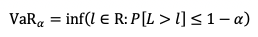
The formula tells us what is the maximum loss we can expect tomorrow, with normal market conditions, or what amount of loss should we not exceed with a given level of probability (e.g. 95%).
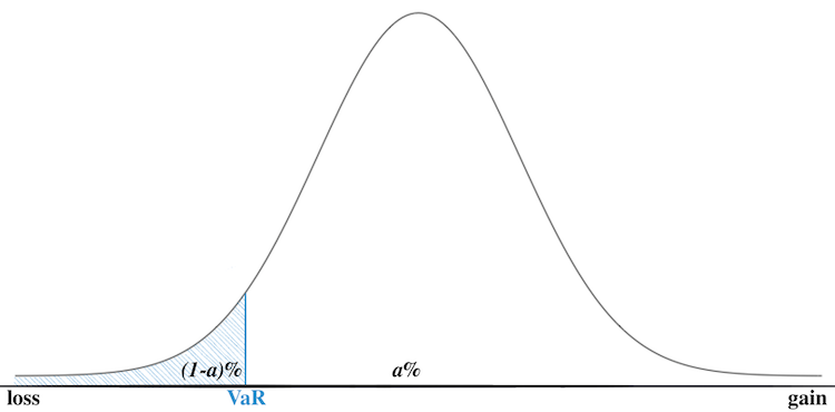
Let’s say a=95% and VaR95%=3%, this tells us there is a 5% chance to lose 3% or more of a portfolio value in a given day. In other words, there is a 95% chance we will not lose more than 3% of portfolio value in a given day, under standard market conditions.
The main pros of VaR are the reaction time, it is easy to use, and it is widely spread, mostly in risk management. However, when looking at tail events (i.e. really negative days), it is less accurate and gives a less precise approximation of a risk compared to the e.g. CVaR (which we will talk about in the next section). To sum up, VaR doesn’t model what happens in the tail, i.e. doesn’t model the tail itself, only the threshold “where the tail begins”.
Calculation
Firstly, there are two main choices to make – the choice of the return distribution model and the choice of the model for volatility. We will examine 3 different models for the distribution of returns and 2 for the volatility. Secondly, we choose 1-day as our loss prediction horizon and 500 days (~2 years) as our historical lookback window. Thirdly, we will be calculating VaR for a=95%.
To make things a little simpler, our portfolio consists of only one asset: SPY ETF. As mentioned, there are many different ways to calculate VaR. We decided to analyse four of the widely used methods:
- Historical simulation
- Parametric Method (assuming Normal distribution)
- Parametric Method combined with GARCH model for volatility
- Monte Carlo simulation combined with GARCH model for volatility
Historical Simulation
The main assumption of this model is that the probability distribution is the same as it was in the previous time period. Then, the calculation is pretty simple and we don’t even need a model for volatility.
In this case, we simply calculate VaR95% as 5th-quantile of the daily returns from the previous period (in our case, previous period = 500 days).
The main benefit of this method is the simplicity and no assumption about the distribution of the risk factors. However, the slow reaction and “jumps” in the case of market turbulence can be a great disadvantage.
The following figure presents daily returns and VaR calculated by this method. We can see the delayed response during times of heightened volatility and also vice versa, when these times end.

Parametric Method
The baseline assumption of all parametric methods is that asset returns do follow a specific distribution. We used Normal distribution in our calculations combined with simple historical volatility, as a model for the volatility. Alternatively, Student’s t-distribution is also widely used (and there are several additional ones as well).
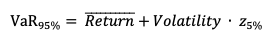
The VaR95% is calculated as a mean return from the previous period (in our case 500 days) plus volatility of the daily returns from the previous period (in our case 500 days) multiplied by 5th-quantile of N(0,1) distribution:
The assumption of a specific distribution is, naturally, never entirely realistic, which is one of the disadvantages of the method. Other disadvantages include slow reaction in turbulent times and the fact that calculating the average value of the past returns is not robust in terms of the selection of the time window.
On the other hand, simplicity is the most significant advantage of this method and, compared to the historical simulation, it’s generally quicker, smoother and more precise.
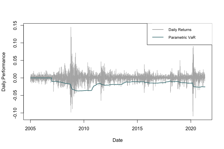
The following figure presents daily returns and VaR calculated by the parametric method using Normal distribution and historical volatility. Again, we can see the late response during times of a heightened volatility (although it’s quicker compared to the historical simulation).
Parametric Method combined with GARCH model for volatility
The third method we applied combines the previous parametric approach with the GARCH model for volatility. As a first step, for each day, we calculate past 20-day GARCH volatility. Then the process is almost identical to the previous method, with the only difference being that instead of using the historical volatility of the daily returns, we use the past 20-day GARCH volatility.
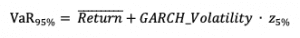
The VaR95% is then calculated as mean return from the previous period (in our case 500 days) plus past 20-day GARCH volatility multiplied by 5th-quantile of N(0,1) distribution:
The main advantage of this method is the GARCH process itself, which depends on past squared returns and past variances to model current variance. As the name suggests, this method is Auto-Regressive and assumes Conditional Heteroskedasticity. This is especially useful because volatility tends to vary in time and is dependent on past variance, making a homoscedastic model suboptimal.
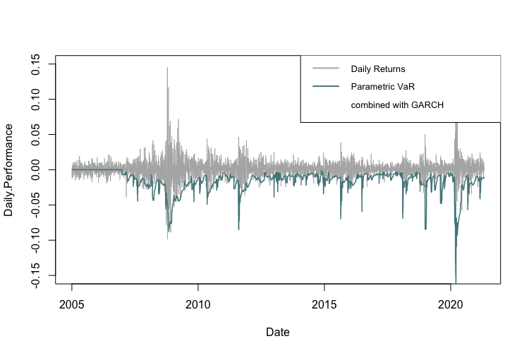
The following figure presents daily returns and VaR calculated by the parametric method using Normal distribution combined with the GARCH model for volatility. This figure shows the fast response to times of heightened volatility.
Monte Carlo simulation combined with GARCH model for volatility
The last method we applied is similar to the previous method, however, instead of using 5th-quantile of N(0,1) distribution we, use Monte Carlo simulations. Each time we generate 500 realizations of a random variable from N(0,1), and subsequently calculate 5th-quantile of these simulations.
The VaR95% is then calculated as mean return from the previous period (in our case 500 days) plus past 20-day GARCH volatility multiplied by 5th-quantile of the generated variables:

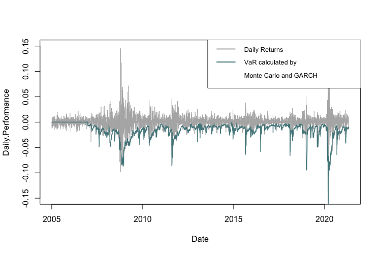
The figure below presents daily returns and VaR calculated by this method. It is evident that the reaction time to the periods of heightened volatility is fast. Nevertheless, a difference between Monte Carlo method and usage of a standard z-score is only marginal, because simulations tend to converge to z-score with the growing number of runs.
Conclusion
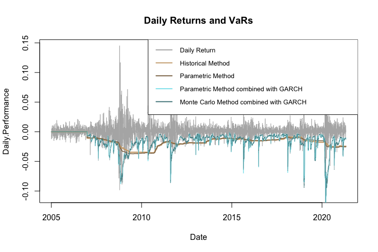
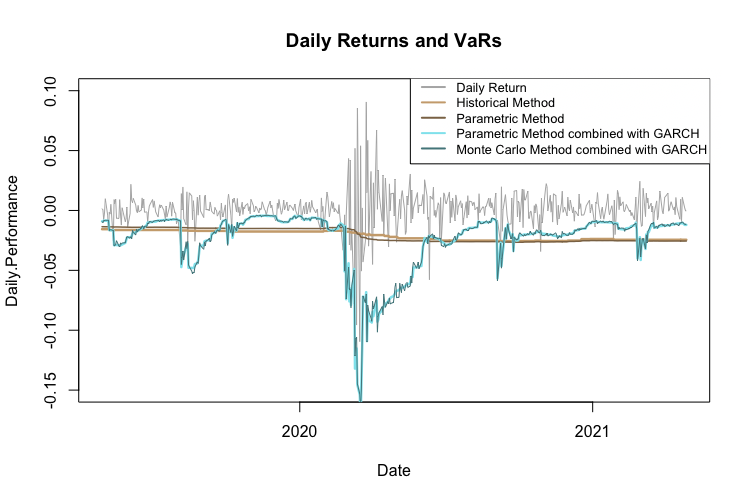
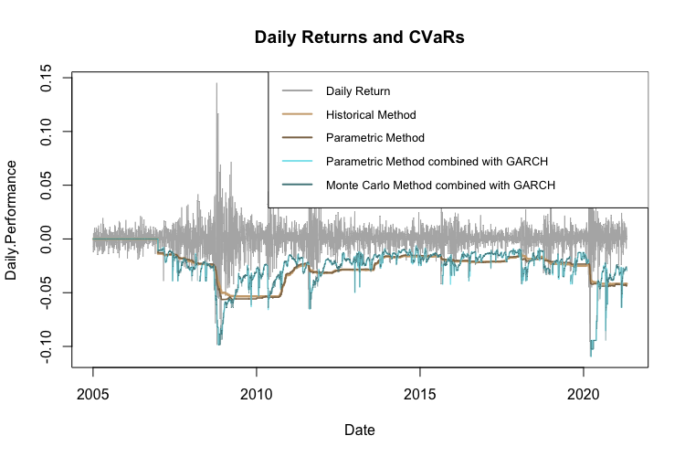
The following figure compares the VaRs calculated by the four different methods. We can clearly see that the methods that use GARCH volatility track the actual loss risk development most closely. Additionally, the difference between the historical method and the parametric method that uses N(0,1) is not that huge. The same applies to parametric method using GARCH compared to the Monter Carlo simulations with GARCH, which are almost identical.
The same chart for the period 2-year period 2019-2021:
| What about Data? Look at Quantpedia’s Algo Trading Discounts. |
Furthermore, VaR can be used to analyse a whole portfolio, not just one asset. The historical and the parametric method work in a very similar manner also in multiple-assets case. However, things get more complicated with multidimensional GARCH and Monte Carlo. We will not cover the multi-asset case, to keep the report brief and clear.
Additionally, there is the possibility to evaluate how well VaR predicts the 5% (or 1-a) probability loss. What we use for such an analysis is the so-called backtesting. The backtesting works on the principle of checking how many times the real loss crossed (was bigger than) the VaR threshold. Numerous statistical tests analyse this, such as Kupiec’s test based on Likelihood Ratio or Christoffersen’s test.
Conditional Value at Risk
Introduction
Conditional Value at Risk (CVaR), also known as the expected shortfall, is defined as a risk assessment measure that quantifies the amount of tail risk an investment portfolio has with a given probability distribution and standard market conditions. In other words – what will be the loss, if the “5% probability loss” occurs?
For example, let’s say a=95% and CVaR95%=4.5%. This tells us that in the worst 5% of the cases, the average loss is 4.5% of the asset value.
Calculation
Just like with VaR, there are multiple ways to calculate CVaR. We analyse the same four methods:
- Historical simulation
- Parametric Method (assuming Normal distribution)
- Parametric Method combined with GARCH model for volatility
- Monte Carlo simulation combined with GARCH model for volatility
Historical Simulation
Assuming that the probability distribution is the same as it was in the previous time period, the calculation is pretty simple. CVaR is the average of the daily returns (in our case, from the past 500 days) that are lower than the VaR value.
The following figure shows the difference between VaR and CVaR calculated by the historical method. Once again, we can see a lag in the reaction to the more volatile time periods.

Parametric Method
There are two ways to approach this method. The first one uses just a simple average below VaR threshold, just like the historical method – but the VaR threshold is calculated according to the parametric method. The second approach involves an exact formula. Let us briefly explain both methods.
The first approach calculates CVaR as the average of the daily returns (in our case, from the past 500 days) that are lower than the VaR value calculated using the parametric method.
The second approach calculates CVaR as a mean daily return (from past 500 days) plus volatility of the returns, times Z:
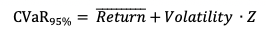
Where
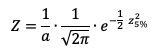
and z is (1-a)th-quantile of N(0,1) distribution.
The following figure compares CVaR calculated by both of the methods and VaR calculated using the parametric method. For the sake of brevity, we will be using only CVaR calculated as the average of the values that are lower than the VaR threshold in all further calculations.

Parametric Method combined with GARCH model for volatility
The third method we applied combines the approach from the previous method with the GARCH model for calculating volatility. Everything is the same as in VaR calculations for this method.
We calculate CVaR as the average of the daily returns (in our case, from the past 500 days) that are lower than the VaR value calculated using the parametric method combined with the GARCH model.
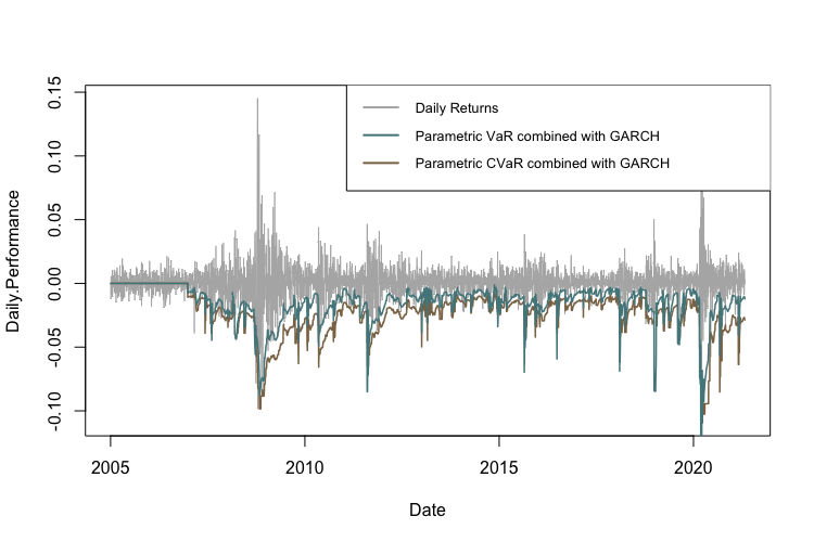
The figure below shows the difference between VaR and CVaR calculated using the parametric method with the GARCH model for volatility.
Monte Carlo simulation combined with GARCH model for volatility
Once again, the last method we applied uses Monte Carlo simulations instead of using (1-a)th-quantile of N(0,1) distribution. Each time we generate 500 realizations of random variable N(0,1) and calculate (1-a)th-quantile of the results.
The CVaR(1-α) is then calculated as the average of the daily returns (in our case, from the past 500 days) that are lower than the VaR value calculated using the same method.
The figure below presents daily returns, VaR and CVaR calculated by this method.

Conclusion
The following figure compares four different CVaR methods. For calculation we use a simple average of the values below correspondent VaR threshold. GARCH volatility seems to be the main deal breaker when it comes to the faster reaction time during volatile periods.
Conditional Drawdown at Risk
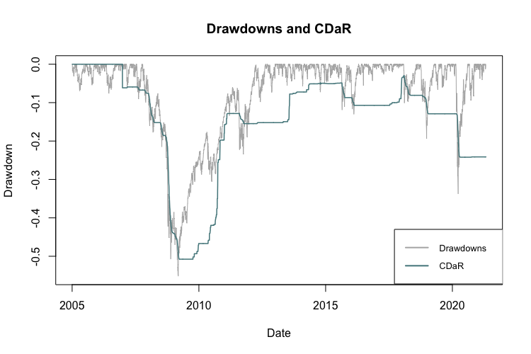
Conditional Drawdown at Risk (CDaR) is defined as the average drawdown for all the occurrences in which the drawdown exceeds a certain threshold. The logic is very similar to CVaR, we’re just using drawdowns instead.
The key assumption is that the probability distribution is the same as in the previous period (in our case, the time period is 500 days). Then the calculation is pretty simple. Firstly, we set a significance level a (in our case a=95%). Secondly, we calculate CDaR95% as the average of the drawdowns from the previous period that are lower than the 5th-quantile of the drawdowns from the previous period.
So, for example, if a=95% and CDaR95% = -16%, this tells us that in the worst 5% of the cases, the average drawdown is -16%.
The following figure shows the drawdowns and the CDaR.
Author:
Daniela Hanicova, Quant Analyst, Quantpedia
Are you looking for more strategies to read about? Sign up for our newsletter or visit our Blog or Screener.
Do you want to learn more about Quantpedia Premium service? Check how Quantpedia works, our mission and Premium pricing offer.
Do you want to learn more about Quantpedia Pro service? Check its description, watch videos, review reporting capabilities and visit our pricing offer.
Do you want algorithmic access to the full Quantpedia database via the API? Subscribe to Quantpedia Pro, ask for an API key, and explore the in/out-of-sample statistics, source academic papers, and code snippets — ideal for quantitative research, systematic trading workflows, and AI model training.
Are you looking for historical data or backtesting platforms? Check our list of Algo Trading Discounts.
Or follow us on:
Facebook Group, Facebook Page, Telegram, Twitter, Linkedin, Medium or Youtube
Share onLinkedInTwitterFacebookRefer to a friend


