An important paper about correlation structure of anomalies:

Authors: Geertsema, Lu

Title: The Correlation Structure of Anomaly Strategies

Link: https://papers.ssrn.com/sol3/papers.cfm?abstract_id=3002797

Abstract:

We investigate the correlation structure of anomaly strategy returns. From an initial 434 anomalies, we select 116 anomalies that are significant in the mean and not highly correlated with other anomalies. Cluster analysis reveals 24 clusters and 29 singleton anomalies that can be grouped into 3 essentially uncorrelated blocks. Correlations between anomaly strategies exhibit some stability over time at both a pairwise and aggregate level. The exception is a correlation spike in 2001, possibly related to the aftermath of the dot-com crisis. In volatile markets correlations increase in magnitude while maintaining their sign. Short and long legs of the same anomaly are highly correlated but becomes largely uncorrelated once we use market excess returns, suggesting that the long and short legs of anomalies follow different dynamics once market-wide influences are compensated for. Correlations based on the residuals of benchmark models are substantially lower, with mean absolute correlation declining by up to half. The existence of 116 anomaly strategies that are not highly correlated echoes other findings in the literature that the return generating process for realised returns appears to be of a high dimension.

Notable quotations from the academic research paper:

"Our paper investigates the correlation structure of 434 anomaly strategies. To our knowledge we are the first to examine the correlation structure of anomaly strategies in detail on this scale. The importance of anomalies may be self-evident to researchers in the field. But what do we gain by investigating the correlation structure of anomalies? We advance three arguments to motivate our work.

First, we argue that the importance of an anomaly should depend on both its magnitude and its uniqueness relative to other anomalies. The magnitude of anomalies is both well studied and well reported. On the other hand, little is known about the uniqueness of a given anomaly relative to the rest. Most anomaly research conduct the usual time-series alpha tests on anomaly portfolios and may, in addition, control for a handful of other anomalies. At one extreme, a new anomaly might be so highly correlated with another anomaly as to essentially constitute the same effect, thus at best contributing a more nuanced understanding or interpretation of the original anomaly. At the other extreme, a new anomaly might be completely orthogonal to all known anomalies. Such an anomaly is clearly more valuable in furthering our understanding of the cross-section of realised returns. The correlation between anomalies allows us to quantify which anomalies are unique, which are related and which are essentially the same, thus imposing a measure of order on the factor zoo.

Second, understanding the correlation structure between anomalies (and its dynamics over time) may aid in uncovering the underlying sources of macro-economic risk that drives the compensation for-risk component of anomaly excess returns. Groups of anomalies that are consistently correlated may point towards common underlying factors, thus aiding in the construction of better expected return benchmark models.

Third, correlation, in combination with asset variance, completely determines the covariance matrix of asset returns. The return covariance matrix has played a central role in virtually all portfolio management since Markowitz.

We find that some anomalies are highly correlated with other anomalies, to the extent that it is very likely that they reflect the same latent effect. Once we restrict ourselves to the 151 anomalies that are significant in the mean, 36% percent of anomalies have an absolute pairwise correlation above 0.8 with some other anomaly. Despite this, 116 anomaly strategies remain even when we consolidate highly correlated anomalies (those correlated at 0.8 or above). A principal component analysis conducted on the 116 anomalies confirms the high-dimensionality of the dataset. A total of 60 principal components are needed to explain 90% of the variation in the 116 anomalies. Many finance researchers have a prior that there should be only a small number of independent sources of priced risk – and certainly not 60. An interpretation that avoids this tension is that much of the outperformance of anomaly strategies may be a combination of a) mispricing and b) data-mining.

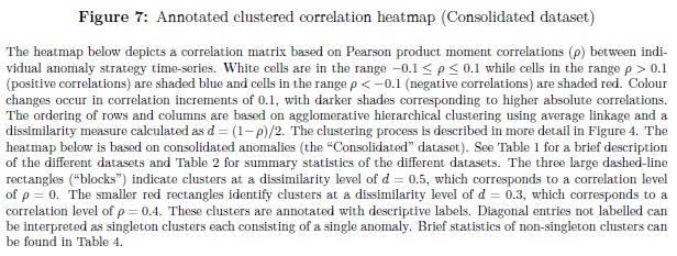
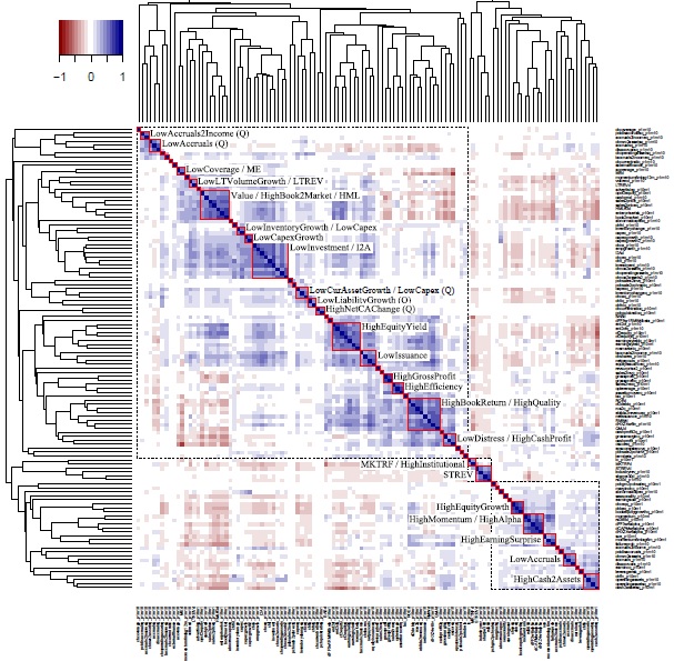
We find clusters of anomalies that exhibit high within-cluster correlation. Between-cluster correlation ranges more widely from positive to negative. Together the pattern is one of intricate correlation structures that appear qualitatively different from either white noise or a simple linear factor data generating process. The anomalies grouped within clusters make sense, in that their similarity is evident from the way in which they are constructed. This enables us to assign to these 24 clusters tentative labels. In addition to the 24 labelled clusters, we also identify 29 “singletons” – single anomalies that can be thought of as clusters containing a single anomaly. At a higher level, we identify three “blocks” of anomalies. The pairwise correlations between anomalies in the same block are almost always positive, while the correlations between anomalies in different blocks are often negative.

Once we eliminate highly correlated anomalies and anomalies that are not significant in the mean, the average correlation between two distinct anomalies is 0.05. This very low average correlation has been cited as a reason why there is no need to control a new anomaly against every single existing anomaly. We find that the mean (across anomalies) of the maximum correlation relative to other anomalies is 0.68, dropping to 0.56 if highly correlated anomalies are consolidated. This suggests that at least some of the new anomalies proposed in the literature may not be as unique as previously thought.

There is evidence that the correlation structure of anomalies are state-dependent. In particular, we find that volatile months (those in the top quartile measured by daily market volatility) produce correlations with substantially higher magnitude but with the same sign as quiet months (those in the bottom quartile). In other words, positive correlations become more positive and negative correlations become more negative in volatile markets. This stands in contrast to the received wisdom that asset correlations tend toward one in volatile markets.

"

Are you looking for more strategies to read about? Check http://quantpedia.com/Screener

Do you want to see performance of trading systems we described? Check http://quantpedia.com/Chart/Performance

Do you want to know more about us? Check http://quantpedia.com/Home/About

A new financial research paper related to:

#75 – Federal Open Market Committee Meeting Effect in Stocks

Authors: Cocoma

Title: Explaining the Pre-Announcement Drift

Link: https://papers.ssrn.com/sol3/papers.cfm?abstract_id=3014299

Abstract:

I propose a theoretical explanation for the puzzling pre-announcement positive drift that has been empirically documented before scheduled Federal Open Market Committee (FOMC) meetings. I construct a general equilibrium model of disagreement (difference-of-opinion) where two groups of agents react differently to the information released at the announcement and to signals available between two announcement releases. In contrast to traditional asset pricing explanations, this model matches key empirical facts such as (1) the upward drift in prices just before the announcement, (2) lower (higher) risk, price volatility, before (after) the announcement occurs, and (3) high trading volume after the announcement, while trading volume is low before the announcement occurs.

Notable quotations from the academic research paper:

"It seems implausible that price increases in the aggregate equity market occur persistently and at scheduled points in time without any associated risk. Still, this was the description of the pre-announcement drift puzzle found in
Lucca and Moench (2015), henceforth LM. The authors documented a persistent upward drift in equity prices together with very low volatility before the scheduled announcements of the FOMC meetings. This paper seeks to provide a theoretical framework to explain how such a positive drift persist and species what kind of risk is embedded in it.Over the past decades, stocks in aggregate have experienced large positive excess returns in anticipation of scheduled FOMC announcements and, to a certain extent, in anticipation of scheduled corporate earnings announcements. I will refer to this phenomenon as the pre-announcement drift. I will claim that, while traditional asset pricing explanations would fail to match the empirical evidence, a model of disagreement based on Dumas et al. (2009), henceforth DKU, creates sentiment risk that matches the stylized facts documented empirically in the literature.

I present a general equilibrium model in which two groups of agents have differences-of-opinion about the content of an announcement. In this economy, there is a continuous stream of dividends being paid, but the rate of growth
of these dividends is unknown and not directly observable. All investors receive information from the current dividend and a signal they may choose to acquire about the unknown growth rate. Agents have different beliefs about the
correlation between their information sources, announcement and signal, and the unobserved rate of growth of dividends. This heterogeneity in the correlation makes the expectations of two groups of agents differ; I will henceforth
call the fluctuations in the beliefs of the two groups as changes in "sentiment". The single parameter in this model that sets it apart from traditional rational-expectations general equilibrium models is the non-zero correlation between the information sources and the unobserved rate of growth. In this model, agents will always have a source of difference-of-opinion because they disagree on a fixed parameter of the model. They, therefore, do not learn from each other's behavior nor from price but simply "agree to disagree".

The intuition of the model in this paper is the following: When an announcement about the unobserved growth rate of the economy occurs, there will be a discontinuous jump in disagreement. This happens because agents will have different interpretations of the information released at the announcement; they assume different correlations of the announcement release and the unknown growth rate. Over time, in the period between announcements, agents will in general remain at a certain level of disagreement, because at least one group of agents acquires a signal about the unobserved growth rate of the economy that the other group of agents does not acquire. Once the next announcement becomes imminent, it would be optimal for all agents to stop acquiring any signal because a new announcement will make all previous information stale. There will be an optimal point in time when the acquiring costs will outweigh the benefits from potentially using the information to be acquired. Therefore, agents will choose not to acquire information, which will bring agents to drastically reduce their disagreement level.

When agents stop acquiring signals, the reduction in disagreement leads to a reduction of sentiment risk that manifests as an increase in prices; this increase in prices will match the pre-announcement drift. Low volatility will be observed in the pre-announcement period, where there is low sentiment risk; and high volatility will be observed after the announcement, where there is an increase in sentiment risk. Finally, high trading volume will occur just after the announcement is released, since this is the point in time with the highest level of disagreement and it would be at its lower point just before the next announcement occurs."

Are you looking for more strategies to read about? Check http://quantpedia.com/Screener

Do you want to see performance of trading systems we described? Check http://quantpedia.com/Chart/Performance

Do you want to know more about us? Check http://quantpedia.com/Home/About

A new interesting research paper related to:

#12 – Pairs Trading with Stocks

Authors: Figuerolla-Ferretti, Serrano, Tang, Vaello-Sebastia

Title: Supercointegrated

Link: https://papers.ssrn.com/sol3/papers.cfm?abstract_id=3005358

Abstract:

This paper uses S&P100 data to examine the performance of pairs trading portfolios that are sorted by the significance level of cointegration between their constituents. We find that portfolios that are formed with highly cointegrated pairs, named as "supercointegrated", yield the best performance reflecting a positive relationship between the level of cointegration and pairs trading profitability. The supercointegrated portfolio also shows superior out-of-sample performance to the simple buy-and-hold investments on the market portfolio in terms of Sharpe ratio. We link the time-varying risk of the pairs trading strategy to aggregated market volatility. Moreover we report a positive risk-return relationship between the strategy and market volatility, which is enhanced during the bear market. Our results remain valid when applying the strategy to European index data.

Notable quotations from the academic research paper:

"This article uses an out-of-sample analysis of S&P100 equity data to analyze performance of pairs trading portfolios when sorted by the level of cointegration of their constituents. We focus on the supercointegrated portfolio, that is formed by pairs in the top quintile of tradable targets, all of which do not reject standard cointegration tests at the 1% significance level. Indeed, the primary contribution of this article is to show that pairs trading profitability is monotonically associated with the significance level of cointegration. For the supercointegrated portfolio, the average excess return of 6.2% is earned per annum which is 2.3% higher than the portfolio with pairs in the second quintile. A similar finding is documented in terms of Sharpe ratio, which increases from 0.2 to 0.6 (yielded by the bottom and the top quintile portfolios, respectively).

A regression of the returns of the supercointegrated portfolio against the 3-factor Fama and French (1992) model shows that the market is a statistically significant explanatory variable of the pairs trading profitability. Momentum and book-to-market ratio are not significant in this exercise. We analyze the sources of risk underlying the supercointegrated portfolio and show that portfolio risk can be linked to aggregate market volatility. We then account for volatility persistence by providing maximum-likelihood estimates of an AR(1) model in the realized volatility series. We find that pairs trading profitability exhibits volatility persistence which is linked to that reported for the market. This allows us to show that lagged market realized volatility can be used to explain current pairs trading profitability. Moreover the strength of the relationship between pairs trading profitability and realized market volatility is positively associated with the level of cointegration underlying pairs trading portfolios. An extended regression analysis demonstrates that the link between realized market volatility and pairs trading profitability is enhanced under bear market conditions. This stronger connection is exclusive to the supercointegrated portfolio.

The empirical evidence provided in this article does therefore suggest that the significance level of cointegration can be used for portfolio ranking purposes. Moreover we show that this evidence is maintained under its application to European equity data. In parallel to our findings, this article conducts several exercises to assess the robustness of its main results. The additional checks conclude, once again, the strength of the supercointegrated portfolio.

."

Are you looking for more strategies to read about? Check http://quantpedia.com/Screener

Do you want to see performance of trading systems we described? Check http://quantpedia.com/Chart/Performance

Do you want to know more about us? Check http://quantpedia.com/Home/About

Out of curiosity, what is benchmark return for each active trader/investor …

Authors: Doeswijk, Lam, Swinkels

Title: Historical Returns of the Market Portfolio

Link: https://papers.ssrn.com/sol3/papers.cfm?abstract_id=2978509

Abstract:

Using a newly constructed unique dataset, this study is the first to document returns of the market portfolio for a long period and with a high level of detail. Our market portfolio basically contains all assets in which financial investors have invested. We analyze nominal, real, and excess return and risk characteristics of this global multi-asset market portfolio and the asset categories over the period 1960 to 2015. The global market portfolio realizes a compounded real return of 4.38% with a standard deviation of 11.6% from 1960 until 2015. In the inflationary period from 1960 to 1979, the compounded real return of the GMP is 2.27%, while this is 5.57% in the disinflationary period from 1980 to 2015. The reward for the average investor is a compounded return of 3.24%-points above the saver’s. We also compare the performance of an investor who holds the market portfolio with an investor who uses simple heuristics for the portfolio allocation. Our results suggest that the market portfolio is close to the mean-variance frontier, but our heuristic allocations achieve a significantly higher reward for risk.

Notable quotations from the academic research paper:

"This study aims to fill both a gap in the academic literature as well as a gap in return data availability for finance practitioners by providing returns of the global market portfolio (GMP) over the period 1960 to 2015 from the perspective of an USD investor. A study on returns of the GMP has not been done before for such a long period and with such a level of detail. We document in detail how we collected historical returns data on global asset classes, which is challenging for the period before 1985. Moreover, we make the resulting data publicly available so other researchers can use them in their own applications. Our GMP basically contains all assets in which financial investors have invested.

This paper contains unique features compared to the scarce academic literature on international asset returns. First, our sample period significantly extends the 1960-1980 period of Ibbotson and Siegel (1983), who are the first with a rigorous study on a global multi-asset market portfolio. They find a nominal compounded return of 8.36% for their so-called world market wealth portfolio over the period 1960-1980. Compared to that study, we focus on assets in which financial investors have actually invested. For example, we do not take farmland into account, as it usually belongs to owners that do not hold it as a financial investment and thereby it is not publicly available.

Second, in comparison with Dimson, Marsh, and Staunton (2002), a groundbreaking study that documents annual returns for equities, government bonds, and treasury bills in sixteen countries for the 101-year period 1900-2000, we include returns for more assets like for example corporate bonds and real estate. Also, we use an all-maturity market capitalization weighted government bonds index instead of a GDP-weighted long term government bonds index. The latter is less useful for representing the performance of the asset class global government bonds. Obviously, the length of their sample period remains unmatched.

New data enables an extensive analysis of return and risk characteristics of the GMP and the asset categories over the period 1960 to 2015. We include conditional analyses on recessionary and inflationary periods. We also compare the performance of an investor who holds the GMP with an investor who uses simple heuristics for the portfolio allocation. By comparing the performance of the GMP with alternative portfolio allocation schemes, we can find out whether the GMP has been a good, if not optimal, portfolio during our 56-year sample period. This analysis will also touch upon mean-reversion across asset classes. Moreover, this new data set provides an opportunity to gauge the difference in return and risk for the average investor and saver."

Are you looking for more strategies to read about? Check http://quantpedia.com/Screener

Do you want to see performance of trading systems we described? Check http://quantpedia.com/Chart/Performance

Do you want to know more about us? Check http://quantpedia.com/Home/About

Related to multiple strategies, mainly to Carry, Volatility Selling and Trend-Following strategies …

Authors: Sepp

Title: Diversifying Cyclicality Risk of Quantitative Investment Strategies (Presentation Slides)

Link: https://papers.ssrn.com/sol3/papers.cfm?abstract_id=2980708

Abstract:

What is the most significant contributing factor to the performance of a quantitative fund: its signal generators or its risk allocators? Can we still succeed if we have good signal generators but poor risk management?

We consider the risk of the skewness and the cyclicality of the key quantitative strategies:
1. Carry strategies
2. Volatility strategies
3. Trend-following strategies

We then present the two approaches for diversification of the cyclicality risk for a master portfolio of these strategies using:
1. Top-down allocation
2. Bottom-up allocation

We illustrate a few examples using back-tested data using systematic quantitative strategies with risk-based allocators.

Notable quotations from the academic research paper:

"

"

Are you looking for more strategies to read about? Check http://quantpedia.com/Screener

Do you want to see performance of trading systems we described? Check http://quantpedia.com/Chart/Performance

Do you want to know more about us? Check http://quantpedia.com/Home/About

Financial variables have become the main driving factors explaining the variation in crude oil returns:

Authors: Adams, Kartsakli

Title: Has Crude Oil Become a Financial Asset? Evidence from Ten Years of Financialization

Link: https://papers.ssrn.com/sol3/papers.cfm?abstract_id=2999717

Abstract:

The financialization of crude oil markets over the last decade has changed the behavior of oil prices in fundamental ways. In this paper, we uncover the gradual transformation of crude oil from a physical to a financial asset. Although economic demand and supply factors continue to play an important role, recent indicators associated with financialization have emerged since 2008. We show that financial variables have become the main driving factors explaining the variation in crude oil returns and volatility today. Our findings have important implications for portfolio analysis and for the effectiveness of hedging in crude oil markets.

Notable quotations from the academic research paper:

"We decompose the total variation of crude oil returns and volatility into three distinctive parts: One part that can be explained by economic fundamental factors, one part that can be explained by financialization variables, and a third which consists of the unexplained variation. While decomposing the returns provides information concerning the main drivers of crude oil as an asset, the volatility decomposition reveals the main factors of risk transmission. We show that the relative importance of economic and financial variables changes over time. In particular, the relative importance of financial variables has changed in such a way that crude oil is now closer to a financial asset than to a real physical asset.

Panel A of Figure 4 shows the decomposition of the total variation in crude oil returns. The fraction of the total variation that can be explained by movements in economic variables is indicated by green shaded areas, the percentage that can be explained by financial variables is indicated by the red shaded areas. The remaining variation is unexplained. The large share of unexplained variation may be due to omitted factors such as geopolitical changes, synchronized OPEC oil production, and disrupting weather events. At a given point in time, the sum over all green and red shaded areas represents the R-squared from a regression of monthly crude oil returns on our set of explanatory variables. To obtain time variation, the regression is moved forward in a 5-year rolling window (60 monthly observations). Two observations follow from Figure 4:

During the pre-financialization period, the contemporaneous variation in our eight regressors explains only a small percentage of the total variation in crude oil returns. After the default of Lehman Brothers, the situation changes dramatically. The same set of regressors now explain almost 60% of the return variation. Among the fundamental variables, economic activity and the change in the dollar exchange rate explain 8% and 12% respectively.

The main drivers behind the variation in oil returns are however the financial variables. In particular, the change in the VIX and the S&P 500 returns are responsible for 29% of the variation.

To illustrate this point, the average fraction explained by each set of variables is shown in Panel B of Figure 4. Since the beginning of the financialization period, the financial variables dominate the economic fundamental variables by a significant amount. Traditional fundamental variables have become relatively less important for predicting crude oil returns while recent financial variables can now predict a large share of the return variation. From this finding we conclude that the behavior of crude oil has become more similar to that of financial assets like equities rather than traditional economic demand and supply drivers.

Financial variables can only explain 11% of the total variation in crude oil returns in the years prior to financialization, the impact grows to 35%, becoming the main drivers behind oil price movements. We estimate an even stronger effect on crude oil volatility where the impact of financial variables grows from 19% in the pre-financialization period to 53% since the failure of Lehman Brothers. Our empirical results indicate that crude oil markets underwent significant changes over the last years. These changes were sufficiently large to transform the very nature of crude oil, away from a physical real asset towards a variable that shows a behavior that is comparable to stocks, bonds, and other financial assets."

Are you looking for more strategies to read about? Check http://quantpedia.com/Screener

Do you want to see performance of trading systems we described? Check http://quantpedia.com/Chart/Performance

Do you want to know more about us? Check http://quantpedia.com/Home/About