Our sucessful Quantopian & Quantpedia Trading Strategy Series continues with a third article, written by Matthew Lee, focused on Reversal During Post-Earnings Announcement Drift (Strategy #238):

https://www.quantopian.com/posts/quantpedia-trading-strategy-series-reversals-in-the-pead
(Click on a "View Notebook" button to read a complete analysis)

What is the logic behind this strategy? Jonathan A. Milian in his paper "Overreacting to a History of Underreaction" explores the possibility that well known cross sectional anomalies can reverse over time. And he picks the premier anomaly – Post Earnings Announcement Drift. He finds that stocks with the most negative previous earnings surprise actually exhibit the most positive returns very shortly after the subsequent earnings announcement.

The academic paper speculates that it seems that due to well-documented history of investors underreacting to earnings news, investors are now overreacting to earnings announcement news. Investors position themselves in alignment with the expectation of the PEAD effect so when the next earnings announcement comes, the overcrowding of investors pushes the market beyond efficient, resulting in the correction of investor sentiment and a negative correlation for firm's earnings news in the following days. However classical PEAD (post-earnings announcement drift) literature examines mainly quarterly portfolio returns while this academic paper focuses on 2-days retun therefore it is probable that PEAD still holds and both anomalies exists concurrently.

Matthew Lee from Quantopian performed an independed analysis of initial findings of Jonathan A. Milian's original academic paper (over a sample period from 2011 – 2016 compared to the Milian's 2003 – 2010). What Matthew found? Overall, he found his results to be consistent with Milian's results for all strategy's holding periods from 2-10 days. The best result was a hold period of 9 or 10 days following the Earnings Announcement, rather than 2 days. Firms in the highest decile of past earnings surprise underperform stocks in the lowest decile by -1.78% over a hold period of 10 days (compared to -1.59% over a hold period of 3 days found in the paper).

So, what is the trading algorithm?

1. Each day, pick stocks in the S&P500 which have Earnings Announcements the next day
2. Go short on stocks in the highest decile of previous earnings surprise, long on stocks in the lowest decile of previous earnings surprise
3. Hold for a period of 10 days, then close the position

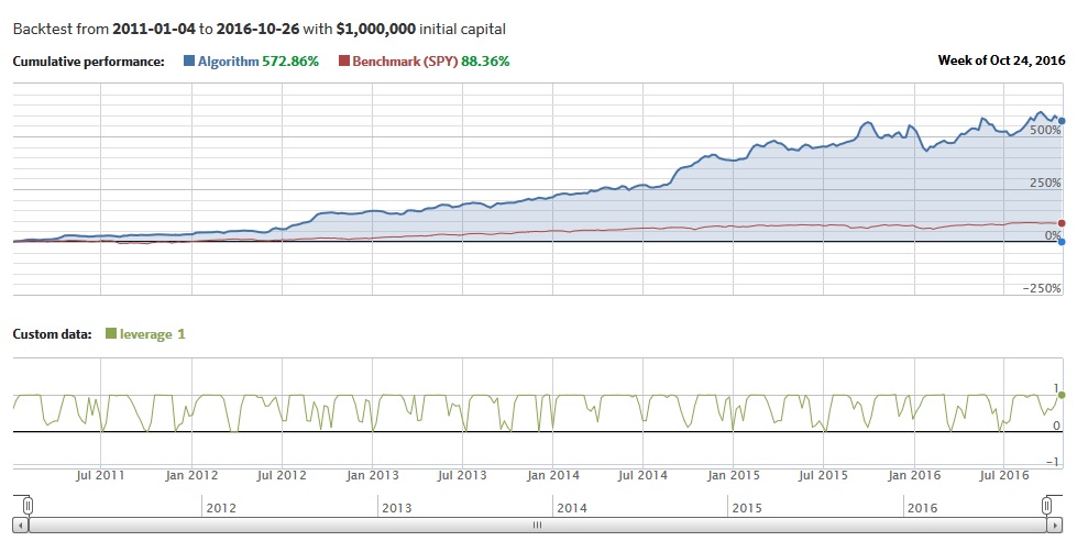
As always, the final OOS equity curve looks really good:

Nice work Matthew!

You may also check first or second article in this series if you liked the current one. And stay tuned for the next …

A related paper has been added to:

#118 – Time Series Momentum Effect

Authors: Dao, Nguyen, Deremble, Lemperiere, Bouchaud, Potters

Title: Tail Protection for Long Investors: Trend Convexity at Work

Link: https://papers.ssrn.com/sol3/papers.cfm?abstract_id=2777657

Abstract:

The performance of trend following strategies can be ascribed to the difference between long-term and short-term realized variance. We revisit this general result and show that it holds for various definitions of trend strategies. This explains the positive convexity of the aggregate performance of Commodity Trading Advisors (CTAs) which — when adequately measured — turns out to be much stronger than anticipated. We also highlight interesting connections with so-called Risk Parity portfolios. Finally, we propose a new portfolio of strangle options that provides a pure exposure to the long-term variance of the underlying, offering yet another viewpoint on the link between trend and volatility.

Notable quotations from the academic research paper:

"In this paper we have shown that single-asset trend strategies have built-in convexity provided its returns are aggregated over the right time-scale, i.e., that of the trend filter. In fact, the performance of trend-following can be viewed as swap between long-term realized variance (typicaly the timescale of the trending filter) and a short-term realized variance (the rebalancing of our portfolio). This feature is a generic property and holds for various filters and saturation levels. While trendfollowing strategies provide hedge against large moves unfolding over the long time scale, it is wrong to expect a 6 to 9 months trending system rebalanced every week to hedge against a market crash that lasts a few days.

We dissected the performance of the SG CTA Index in terms of a simple replication index, using and un-saturated trend on equi-weighted pool of liquid assets. Assuming realistic fees, and fitting only the time-scale of the filter (found to be of the order of 6 months) we reached a very strong correlation (above 80%) with the SG Index, and furthermore fully captured the average drift (i.e. our replication has the same Sharpe ratio as the whole of the CTA industry). However, our analysis makes clear that CTAs do not provide the same hedge single-asset trends provide: some of the convexity is lost because of diversification. We however have found that CTAs do offer an interesting hedge to Risk-Parity portfolios. This property is quite interesting, and we feel it makes the trend a valid addition in the book of any manager holding Risk Parity products (or simply a diversified long position in both equities and bonds).

Finally, we turned our attention to the much discussed link between trend-following and long-volatility strategies. We found that a simple trend model has exactly the same exposure to the long-term variance as a portfolio of naked strangles. The difference is the fact that the entry price of the latter is fixed by the implied volatility, while the cost of trend is the realized short-term variance. The pay-off of our strangle portfolio is model-independent and coincides with that of a traditional variance swap – except that the latter requires Back-Scholes assumptions. In other words, the option strategy is a better hedge and therefore its price should be higher than realized volatility.  The premium paid on option markets is however oo high in the sense that long-vol portfolios have consistently lost money over the past 2 decades, while trend following strategies have actually posted positive performance. So, even if options provide a better hedge, trend following is a much cheaper way to hedge long-only exposure.

All-in-all, our results prove that trending systems offer cheap protection to long-term large moves of the market. This coupled with the high statistical significance of this market anomaly, really sets trend-following apart in the world of investments strategies. A potential issue might be the global capacity of this strategy, but recent performance seems to be quite in line with long-term returns, so there is at presence little evidence of over-crowding."

Are you looking for more strategies to read about? Check http://quantpedia.com/Screener

Do you want to see performance of trading systems we described? Check http://quantpedia.com/Chart/Performance

Do you want to know more about us? Check http://quantpedia.com/Home/About

A related paper has been added to:

#12 – Pairs Trading with Stocks

Authors: Donninger

Title: Is Daily Pairs Trading of ETF-Stocks Profitable?

Link: https://papers.ssrn.com/sol3/papers.cfm?abstract_id=2816288

Abstract:

Pairs trading is a venerable trading strategy. There is agreement that it worked fine in the far past. But it is less clear if it still profitable today. In this working paper the universe of eligible pairs is defined by the holdings of a given ETF. It is shown that the stocks must be from ETFs which select high-quality, low-volatility stocks. The usual closeness measure presented in the literature performs poor. The paper presents a simple and clearly superior alternative based on zero-crossings. The strategy performs with the correct universe and the improved pairs selection rule before trading costs quite fine. It depends on the assumed trading costs if this is also in real-trading life the case.

Notable quotations from the academic research paper:

"The seminal paper on pairs trading is Gatev et. al. [1]. They authors did not invent the strategy. It was in common use since the 1980s. The pairs are formed from a universe of stocks. There is a one year formation period. Each stock is normalized to 1 at the beginning of this period. One selects for each stock the closest neighbor. The distance measure is the summed up squared daily difference of the normalized prices.

The initial results with the distance method were rather disappointing. Pairs trading is based on mean-reversion. The distance measures if the stocks stick together. But sticking together and mean-reversion are two different concepts. Vidyamurthy proposes zero-crossings as an alternative. One counts the number of times the spread moved above or below the mean-spread. But this measure is also not satisfactory. It is known from the theory of Brownian-motions that zero-crossings are much more likely in the first few steps of the motion. If one starts at zero a small up- followed by a larger down-move is a zero crossing. The path moves in the following away from zero and a crossing gets very unlikely. The situation is somewhat different for a mean-reverting process but the general behavior is still the same. A zero (or mean) crossing does also not create a profit. The interesting case is a crossing which started initially outside the two-sigma band. This is the main distance function. A larger number of crossings is of course better than a lower one. For two pairs with the same number of crossing the distance is used as a secondary measure. But a pair with 5 crossings is always closer than a pair with only 4. The strategy defines also a minimum number of crossings (usually 4). A pair with less crossings is never traded.

The strategy does not use overlapping formation periods. The set of tradeable pairs is determined each month (every 21 trading days). The formation window is like in most studies a year (252 trading days). But an open position is not automatically closed at the end of the trading period. An open position is – if mean reversion does not happen before – closed after 30 trading days. There are usually pairs from the previous formation period open. It makes no sense to close a position which was entered at day 20 of the trading period just because a new formation calculation is performed. The strategy does not reset the spread to zero at the end of the formation phase. It uses the mean and the standard deviation from the formation period also in the trading phase. A position is only opened, if the spread is between 2 and 4 standard deviations. It is unlikely that the spread is by chance larger than 4 deviations. A very large spread is a sign that the pair is in divorce. As an additional stop-loss an already open position is closed if the spread gets larger than 8 standard deviations. This stop-loss is only triggered a few times but it avoids some
really disastrous losses.

As already noted simulated trading is done from 2011-01-01 till 2016-07-26. The strategy has an overall profit of 144.4%, a monthly Sharpe ratio of 1.16 and a max. relative drawdown of 8.2%."

Are you looking for more strategies to read about? Check http://quantpedia.com/Screener

Do you want to see performance of trading systems we described? Check http://quantpedia.com/Chart/Performance

Do you want to know more about us? Check http://quantpedia.com/Home/About

A related paper has been added to:

#12 – Pairs Trading with Stocks

Authors: Do, Faff

Title: Cointegration and Relative Value Arbitrage

Link: http://papers.ssrn.com/sol3/papers.cfm?abstract_id=2826190

Abstract:

We examine a new method for identifying close economic substitutes in the context of relative value arbitrage. We show that close economic substitutes correspond to a special case of cointegration whereby individual prices have approximately the same exposure to a common nonstationary factor. A metric of closeness constructed from the cointegrating relation strongly predicts both convergence probability and profitability in cointegration-based pairs trading. From 1962 to 2013, a strategy of trading cointegrated pairs of near-parity generates 58 bps per month after trading costs, experiences a 71% convergence probability and outperforms a strategy of pairs selected by minimized price distances.

Notable quotations from the academic research paper:

"In the pairs trading literature, the most common type of relative value arbitrage, substitutes for individual stocks are identified by minimizing the Euclidean distance in the daily price space over a historical period.5 Matching stocks over the price space instead of the return space is consistent with short-term relative value trading strategies, while removing the need to specify factors. Although the matching method is simple to perform, by design, it guarantees the existence of a counterpart for every stock, which is counterintuitive. More importantly, stocks that exhibit little variation in the price pattern over the formation period (possibly due to lack of news flow) would end up being labelled close substitutes, although they are not fundamentally related.

In this paper, we propose a simple method of identifying close economic substitutes using cointegration. When a pair of stock prices is cointegrated, one series co-moves with a scaled version of the other. We show that close economic substitutes can be represented by a system of cointegrated prices where the scaling factor, or the cointegration coefficient, is close to one.

We find that from 1962 to 2013, NonParity, a positive-valued metric of closeness that measures the distance of the cointegration coefficient from unity, strongly predicts both the probability that relative mispricing will subsequently be corrected as well as the profitability of the arbitrage trade. A one standard deviation increase in the variable reduces the convergence probability by seven percentage points and pairs trade payoffs by 2.78 percentage points. Further, predictability through NonParity also presents profitable trading opportunities. At the portfolio level, the pairs trading of cointegrated stocks is generally unprofitable. However, when trading is confined to pairs of stocks with NonParity close to zero, the strategy is profitable after reasonable estimates of brokerage, slippage, and short selling costs. Specifically, over the sample period, the average after-cost risk-adjusted return to trading a portfolio of cointegrated pairs with NonParity less than 0.5 (0.2) is 0.43% per month, with a t-statistic of 5.29 (0.58% per month, with a t-statistic of 4.77)."

Are you looking for more strategies to read about? Check http://quantpedia.com/Screener

Do you want to see performance of trading systems we described? Check http://quantpedia.com/Chart/Performance

Do you want to know more about us? Check http://quantpedia.com/Home/About

We at Quantpedia consider ourselves a history freaks as we love books and papers related to a history of finance. The work of Dotsis is a perfect example of an interesting paper about a history of option pricing and shows how people were remarkably skilled in assessing price of options even without current high performance IT tools. Academic paper could be related to #20 – Volatiity Risk Premium Effect …

Authors: Ghoddusi

Title: Option Pricing Methods in the Late 19th Century

Link: http://papers.ssrn.com/sol3/papers.cfm?abstract_id=2831362

Abstract:

This paper examines option pricing methods used by investors in the late 19th century. Based on the book called “PUT-AND-CALL” written by Leonard R. Higgins in 1896 and published in 1906 it is shown that investors in that period used routinely the put-call parity for option conversion and static replication of option positions, and had developed no-arbitrage pricing formulas for determining the prices of at-the-money and slightly out-of-the-money and in-the-money short-term calls and puts. Option traders in the late 19th century understood that the expected return of the underlying does not affect the price of an option and viewed options mainly as instruments to trade volatility.

Notable quotations from the academic research paper:

"In this paper I show that option traders in the late 19th century not only had an intuitive grasp of the main determinants of option prices but they have also developed no-arbitrage pricing formulas for determining their prices. The option pricing formulas are described in a book called “PUT-AND-CALL” written by Leonard R. Higgins in 1896 and published in 1906.2 Higgins was an option trader in London and in his book he describes option pricing methods and option strategies used in the late 19th century in the City of London.

The pricing approach described in Higgins book could be summarized as follows: First, traders were pricing short-term ATMF straddles (30, 60 or 90 days to maturity. The prices of the ATMF straddles were set equal to the risk-adjusted expected absolute deviation (Higgins uses the term average fluctuation) of the underlying price from the strike price at expiration. The expectation of the absolute deviation was based on historical estimates plus a risk premium for future uncertainty as well as some other markups. Given the ATMF straddle prices as reference points Higgins is using a linear approximation formulae based on put-call parity to price slightly out-of-the-money (OTM) and slightly in-the-money (ITM) put and call options. I show that the approximation used by Higgins is analogous to a first order Taylor expansion around the ATMF straddle price.

Higgins’s book is an important reference in the history of option pricing because it provides a pricing framework based on empirical rules and approximation methods for determining option prices. Higgins’s method could be taught in introductory derivatives valuation courses before the Black and Scholes and the binomial model to help students appreciate the historical development of option pricing methods and the contribution of option market practitioners."

Are you looking for more strategies to read about? Check http://quantpedia.com/Screener

Do you want to see performance of trading systems we described? Check http://quantpedia.com/Chart/Performance

Do you want to know more about us? Check http://quantpedia.com/Home/About

Related to:
#6 – Volatility Effect in Stocks – Long-Short Version

Authors: Driessen, Kuiper, Beilo

Title: Does Interest Rate Exposure Explain the Low Volatility Anomaly?

Link: http://papers.ssrn.com/sol3/papers.cfm?abstract_id=2831157

Abstract:

We show that part of the outperformance of low volatility stocks can be explained by a premium for interest rate exposure. Low volatile portfolios have a positive exposure to interest rates, whereas the more volatile stocks have a negative exposure. Incorporating an interest rate premium explains part of the anomaly. Depending on the methodology chosen the reduction of unexplained excess return is between 20% and 80%. Our results provide evidence that interest rate risk is priced differently in the bond and equity market. Our results imply a strong implicit exposure of low volatility portfolios to bonds.

Notable quotations from the academic research paper:

"A relation between the low volatility anomaly and government bonds makes sense if volatility is thought of as an indicator of how far equity is removed from bonds in the capital structure. In this study our main finding is that the outperformance of low volatility stocks can be explained by differences in interest rate exposure. We find that low volatility portfolios have more exposure to this risk. Our results imply a strong implicit exposure to interest rate risk of low volatility portfolios. We estimate that the duration of the lowest volatility decile corresponds to a 30% weight to bonds. The duration of the highest decile corresponds to a short position of 100% short bonds.

Because of the differences in exposure, the risk premium that we estimate explains part of the excess return of a long short portfolio. We find a monthly compensation of interest rate risk in equities of 0.91%, with a standard error of 0.20%. The differences in interest rate exposure combined with the large estimated risk premium, results in a significantly reduced mispricing of low volatility stocks. We find these results to be robust for taking into account the time variance of the interest rate exposure.

For our study we use ten portfolios over the period from July 1963 to December 2014, defined by sorts on residual variance of individual US stocks using the Fama French 3 factor model. In section 3 we elaborate further on this. We define an interest rate factor as the return of an equal weight portfolio consisting of US government bonds with various maturities. In order to estimate the interest rate exposure we run time series regressions. Fama MacBeth regressions are employed to estimate the premium for the interest rate exposure. Combined these two enable us to evaluate the impact of this effect on the unexpected excess return of the long short portfolio. We use several different estimations of the premium in order to test the robustness of our findings."

Are you looking for more strategies to read about? Check http://quantpedia.com/Screener

Do you want to see performance of trading systems we described? Check http://quantpedia.com/Chart/Performance

Do you want to know more about us? Check http://quantpedia.com/Home/About