Hedging Tail Risk with Robust VIXY Models
Extreme market events, once perceived as statistical outliers, have become a central concern for investors. The persistence of sharp drawdowns and volatility spikes demonstrates that the cost of ignoring tail risks is not tolerable for long-term portfolio resilience. While diversification can mitigate ordinary fluctuations, it often fails when markets move in unison under stress. This makes explicit protection against severe downside events not just desirable but necessary. Tail hedging addresses this need by providing a structured defense against the most damaging scenarios, ensuring that portfolios remain robust when traditional risk management tools fall short. Using VIXY ETF, we will present and test a range of hedging strategies designed to protect portfolios under stress. By applying robust testing frameworks, we aim to evaluate how different implementations of VIXY ETF-based tail hedges perform across a variety of market environments, highlighting both their strengths and inherent trade-offs.
VIX, VXV & VIXY
In our analysis, we will use the ProShares VIX Short-Term Futures ETF (VIXY) as the primary hedging instrument, combined with the SPDR S&P 500 ETF (SPY) as the core equity exposure. This pairing allows us to explore how volatility-linked assets can mitigate drawdowns in a traditional equity portfolio. To guide the allocation of VIXY within the portfolio, we will incorporate signals derived from the VIX and VXV indices. While these indices cannot be traded directly, their informational value makes them useful modeling variables for determining when and to what extent volatility exposure should be applied. Importantly, only SPY and VIXY will form the investable portfolio, with VIX and VXV serving strictly as inputs to allocation models rather than direct holdings.
The CBOE Volatility Index (VIX) is the most widely recognized measure of expected equity market volatility. Derived from S&P 500 options, the VIX reflects the market’s consensus on near-term uncertainty and is often referred to as the “fear gauge.” Sharp increases in the VIX typically coincide with market stress, making it a natural reference point for tail risk hedging. However, as a non-tradable index, investors cannot directly buy or sell the VIX itself, which limits its use to signaling rather than execution.
The CBOE 3-Month Volatility Index (VXV) extends the concept of the VIX by measuring implied volatility over a three-month horizon. This longer tenor makes VXV less sensitive to short-lived spikes but more reflective of sustained market uncertainty. As a result, the relationship between VIX and VXV is often used as a gauge of market stress regimes, with a rising VIX relative to VXV signaling elevated short-term fear. For tail hedging, VXV provides valuable context by anchoring short-term volatility within a broader temporal framework.
The ProShares VIX Short-Term Futures ETF (VIXY) offers investors a liquid, tradable vehicle to gain exposure to VIX futures. By holding a rolling position in front-month and second-month futures, VIXY seeks to track short-term changes in expected volatility. Its responsiveness to market shocks makes it a practical instrument for implementing tail hedging strategies. Nonetheless, investors must account for structural challenges such as roll costs in contango environments, which can erode value over time. Despite these limitations, VIXY remains one of the most accessible tools for translating volatility expectations into actionable hedges. This asset was introduced in 2011, so to have a longer data history, we reconstructed it previous history since 2004 until 2011 using VIX futures.
Benchmark strategy
A simple yet powerful signal for timing VIXY exposure arises from the relationship between the short-term VIX and the medium-term VXV. Under normal market conditions, the VIX, which reflects 30-day implied volatility, tends to be lower than VXV, the 90-day measure. This reflects the market’s expectation that immediate uncertainty is usually smaller than medium-term uncertainty, a typical feature of stable markets.
When market stress emerges, the usual relationship can invert: the VIX rises above VXV, signaling that short-term fear exceeds medium-term expectations. For VIXY, which tracks short-term VIX futures, this inversion is particularly meaningful. It identifies periods in which the ETF is likely to respond sharply to spikes in volatility, making it an efficient hedge precisely when equity markets face the greatest risk. By using this signal, investors can avoid the costs of holding VIXY continuously and instead activate exposure only when it is most likely to be effective.
Following this strategy, we will allocate up to 20% of the portfolio dynamically to VIXY, with the remainder, 80%, held in SPY. The VIXY allocation is conditional: it is either fully invested according to the signal or held in cash when the signal does not trigger. Importantly, the allocation updates occur with a one-day lag. This is because we rely on VIX and VXV values from the previous market close, and trades are executed at the close of the following day. This timing ensures that the strategy remains implementable in practice while accurately reflecting the information provided by the volatility signals.
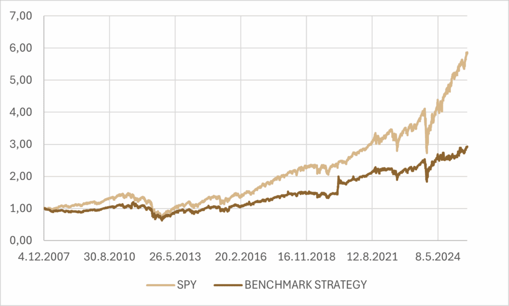
Table 1: Performance metrics of 100% SPY and 20% VIX-VXV signal for VIXY and 80% SPY strategy.
| PORTFOLIO | CAR p.a. | VOL p.a. | SHARPE |
|---|---|---|---|
| 100% SPY | 10.52% | 18.71% | 0.56 |
| 80% SPY, 20% VXV-VIX signal for VIXY | 6.25% | 16.29% | 0.38 |
While the VIXY-hedged portfolio demonstrates a reduction in absolute risk, its lower return and Sharpe ratio relative to the SPY benchmark suggest that, at least over the period considered, the hedge comes at a cost that is not fully offset by improved risk-adjusted performance. This highlights a key challenge in tail hedging: while protection against extreme events is valuable, it can reduce overall efficiency if the signal is too conservative or market conditions do not frequently trigger significant drawdowns. As such, the benchmark itself does not appear sufficiently effective in capturing the potential benefits of the hedge, underscoring the need for careful strategy design and robust testing. Therefore, there is a clear need to explore improved approaches that balance downside protection with overall portfolio efficiency.
Previous research
We have already covered the question of selective hedging using the triple leveraged ETFs in which we were inspired by Carlo Zarattini, Antonio Mele, and Andrew Aziz previously published article addressing this very topic, which provides an excellent starting point for our analysis. In their work, they presented multiple tail hedging strategies, covering a wide range of approaches and implementation styles. For the purposes of this article, we will narrow our focus specifically to long-only strategies, examining how they perform under different market conditions. Beyond simply implementing these strategies, our goal is to rigorously test their robustness, assessing not only their effectiveness in reducing downside risk but also their consistency and practical viability over time. The article introduces two strategies that form the basis of our discussion.
All strategies presented involve a concept of expected volatility risk premium. The expected volatility premium is calculated as the difference between the implied volatility of VIX or VXV at time t and the realized volatility of the underlying asset, in this case the S&P 500, over the corresponding horizon T. In other words, it measures how much the market’s expectation of future volatility exceeds the actual observed variability of the index.
The second indicator employed in both strategies is the smoothing of VIX or VXV values. This approach involves comparing the current level of the index to a moving average calculated over the past several days (in case of this article, it is 90 calendar days). By doing so, the strategy captures short-term deviations from recent trends, helping to identify periods when volatility is unusually high or low relative to its recent history.
This approach integrates relatively well with the benchmark, as it similarly allocates 20% to a hedging strategy.
This approach represents what is commonly referred to as “sizing,” which involves allocating a larger portion of capital to the hedging asset as market uncertainty increases. In practice, given the fixed allocation proportions discussed earlier, this means that during periods of exceptionally high uncertainty, it may be necessary to employ leverage on a short-term basis to maintain the desired exposure. The costs associated with such leverage are ignored in this analysis, as these positions are typically very short-lived and quickly adjusted once market conditions normalize.
Let’s get back to basics
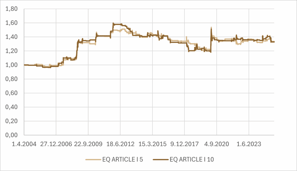
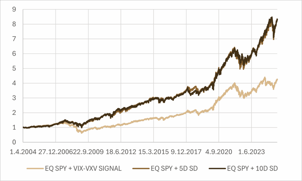
In the previous section, we introduced two strategies that will be the focus of our analysis. To begin, we will start with the simpler one: the version without sizing. Here, the hedge allocation is capped at 20% of the portfolio, but it is activated only when the conditions of the signal are met, namely when the expected volatility risk premium (eVRP) is less than or equal to zero and the VIX exceeds its three-month moving average (VIX3M). Outside of these conditions, the hedge remains in cash. This framework represents a fixed-weight implementation of the strategy and provides a useful baseline for evaluating its effectiveness before moving on to the more complex version with dynamic sizing.
Let us now examine whether this strategy is truly robust or whether its performance may simply be the result of chance. To address this question, we can vary the parameters that define the signals. Specifically, we will experiment with the window length used to calculate the standard deviation of the S&P 500, as well as the smoothing window applied to VIX. By testing the strategy across different parameter settings, we can evaluate the consistency of its results and determine whether its effectiveness holds up beyond a single calibration.
Table 2: Sensitivity of annualized yields to eVRP and moving average window length, MA windows in trading days are 2/3 of calendar days, execution shifted by 1 day, calculated between 01.04.2004 and 31.07.2025.
| eVRP | 10 D | 20 D | 30 D | 40 D | 60 D | 80 D | 90 D | 100 D | 120 D |
|---|---|---|---|---|---|---|---|---|---|
| 5 | 0.70% | 1.68% | 1.81% | 1.23% | 0.90% | 1.23% | 1.02% | 0.94% | 0.70% |
| 10 | 0.70% | 1.68% | 1.81% | 1.23% | 0.90% | 1.23% | 1.02% | 0.94% | 0.70% |
| 20 | 0.11% | 0.88% | 1.09% | 0.57% | 0.56% | 1.10% | 0.93% | 0.91% | 0.75% |
| 30 | -0.94% | 0.09% | 0.22% | -0.47% | -0.32% | 0.37% | 0.36% | 0.28% | -0.05% |
| 40 | -0.52% | 0.16% | 0.18% | -0.12% | 0.18% | 0.93% | 0.97% | 0.93% | 0.66% |
| 60 | -1.18% | -0.47% | -0.59% | -0.65% | -0.57% | -0.10% | -0.11% | -0.30% | -0.61% |
Table 3: Sensitivity of annualized volatility to eVRP and moving average window length, MA windows in trading days are 2/3 of calendar days, execution shifted by 1 day, calculated between 01.04.2004 and 31.07.2025.
| eVRP | 10 D | 20 D | 30 D | 40 D | 60 D | 80 D | 90 D | 100 D | 120 D |
|---|---|---|---|---|---|---|---|---|---|
| 5 | 3.49% | 4.30% | 4.56% | 4.81% | 5.02% | 5.16% | 5.15% | 5.18% | 5.19% |
| 10 | 3.49% | 4.30% | 4.56% | 4.81% | 5.02% | 5.16% | 5.15% | 5.18% | 5.19% |
| 20 | 2.38% | 2.71% | 2.88% | 3.27% | 3.78% | 4.00% | 4.08% | 4.18% | 4.27% |
| 30 | 2.03% | 2.09% | 2.12% | 2.30% | 2.88% | 3.36% | 3.51% | 3.59% | 3.66% |
| 40 | 2.07% | 1.59% | 1.61% | 1.54% | 2.17% | 2.80% | 3.00% | 3.10% | 3.18% |
| 60 | 2.77% | 1.85% | 1.61% | 1.52% | 1.30% | 1.51% | 1.79% | 1.92% | 2.19% |
Table 4: Sensitivity of Sharpe to eVRP and moving average window length, MA windows in trading days are 2/3 of calendar days, execution shifted by 1 day, calculated between 01.04.2004 and 31.07.2025.
| eVRP | 10 D | 20 D | 30 D | 40 D | 60 D | 80 D | 90 D | 100 D | 120 D |
|---|---|---|---|---|---|---|---|---|---|
| 5 | 0.20 | 0.39 | 0.40 | 0.26 | 0.18 | 0.24 | 0.20 | 0.18 | 0.14 |
| 10 | 0.20 | 0.39 | 0.40 | 0.26 | 0.18 | 0.24 | 0.20 | 0.18 | 0.14 |
| 20 | 0.05 | 0.32 | 0.38 | 0.17 | 0.15 | 0.28 | 0.23 | 0.22 | 0.18 |
| 30 | -0.46 | 0.04 | 0.10 | -0.20 | -0.11 | 0.11 | 0.10 | 0.08 | -0.02 |
| 40 | -0.25 | 0.10 | 0.11 | -0.08 | 0.08 | 0.33 | 0.32 | 0.30 | 0.21 |
| 60 | -0.43 | -0.25 | -0.37 | -0.43 | -0.44 | -0.06 | -0.06 | -0.15 | -0.28 |
The results in the previous table suggest that the 10-day moving average window provides a consistent and robust estimate. Sharpe ratios, return and volatility values remain stable across different testing horizons, while avoiding the pronounced negative outcomes that may emerge for longer windows. Choosing a 10-day window therefore represents a balanced compromise: it is short enough to capture relevant short-term market dynamics, but long enough to filter out excess noise that would otherwise dominate at even shorter intervals. In the following sections, we will therefore focus exclusively on the 5 and 10-day window and examine its behavior under varying market conditions and with respect to complementary performance measures.
It is important to note that throughout our analysis, the strategy is implemented with a one-day execution lag. In practice, both the eVRP signal and the moving average are evaluated with a delay of one trading day. This reflects the operational constraint that it is not feasible to open or close positions instantaneously at the post-market stage once the signal has been generated.
By applying this lag consistently, we ensure that the results reflect a realistic trading framework rather than an idealized setup that would be difficult to replicate in practice. While this adjustment slightly reduces the theoretical efficiency of the signals, it provides a more robust and implementable measure of strategy performance.
For completeness, we also evaluated all strategies without applying the one-day execution lag. The results indicate that the strongest signals were captured equally well, regardless of whether the lag was present. The main differences were limited to marginal variations in overall performance and risk measures.
This finding reinforces the robustness of the signals themselves: the choice between implementing or omitting the execution lag primarily affects the practical execution profile rather than the underlying informational content. In other words, the lag introduces only a modest trade-off between theoretical efficiency and realistic implementability, without altering the fundamental conclusions about the strategies’ effectiveness.
Is our model overfitted?
It is worth noting that our approach might be slightly aggressive in what we consider a “signal.” We focus on very specific indicators, and there is a risk of overfitting if we try to extract too much from market data. For example, attempts to smooth the VIX curve may go beyond reasonable analysis and verge on over-optimization.
So, if we just avoid this condition and focus solely on eVRP < 0, we can obtain a new benchmark.
Similarly, we can ask whether eVRP could also be considered using VXV as a basis. Let us explore this possibility and create a new benchmark based on it.
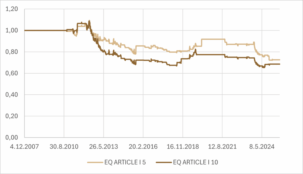
Table 5: Performance metrics of benchmark and modified article strategies.
| PORTFOLIO | CAR p.a. | VOL p.a. | SHARPE |
|---|---|---|---|
| 20% VIX-VXV signal for VIXY | -2.13% | 6.43% | – |
| 20% VIX 5D eVRP signal for VIXY | 1.79% | 5.86% | 0.32 |
| 20% VIX 10D eVRP signal for VIXY | 1.70% | 5.71% | 0.30 |
| 20% VXV 5D eVRP signal for VIXY | -1.80% | 5.46% | – |
| 20% VXV 10D eVRP signal for VIXY | -2.12% | 5.29% | – |
We can see that choosing the signal based on 5-day or 10-day eVRP works well, but only when we use VIX as the underlying measure—not VXV. At the same time, it becomes clear that our benchmark performs rather poorly, which further highlights the importance of carefully defining the reference point. Another important observation is that article strategies perform better in terms of returns, but in terms of risk adjusted returns, modified strategies have better Sharpe ratio.
Sizing as the key to improved performance
In the previous section, our findings regarding the exclusion of smoothing in the VIX eVRP signal were somewhat inconclusive. We will still keep strategies based on just the VIX eVRP signal in consideration, as we did not combine them with SPY in 80/20 portfolio yet. However, the original article we followed proposed an additional refinement: adjusting position sizing in proportion to the level of VIX.
In these strategies, we keep the same signal as before, but the portfolio weight is no longer fixed. Instead, it is determined by the current level of the VIX. For example, if the VIX is at 28, the allocation to VIXY in the portfolio at that time would be 28%. Naturally, this means that when combined with, say, an 80% allocation to SPY, the portfolio weight can exceed 100%, requiring the use of leverage. In this analysis, we ignore the costs of leverage, as these positions are intended to be short-term.
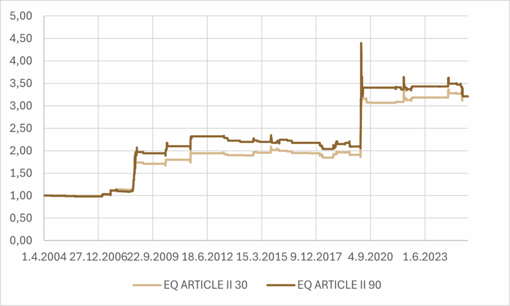

Table 6: Performance metrics of modified article strategies using sizing.
| PORTFOLIO | CAR p.a. | VOL p.a. | SHARPE |
|---|---|---|---|
| 5D SD & 30D MA for VIX strategy | 6.55% | 11.91% | 0.55 |
| 5D SD & 90D MA for VIX strategy | 7.18% | 12.85% | 0.56 |
| 10D SD & 30D MA for VIX strategy | 6.55% | 11.91% | 0.30 |
| 10D SD & 90D MA for VIX strategy | 7.18% | 12.85% | 0.56 |
What we can observe is that the behavior under both window choices, whether 5-day or 10-day, is essentially identical. Once again, we can see that these strategies are relatively robust, so from this point onward we will work only with the 10-day standard-deviation version.
The results we obtained exhibit significantly improved characteristics compared not only to the benchmark strategies but also to the variants without dynamic sizing and to those that excluded smoothing. In other words, incorporating VIX-based proportional sizing provides a clear enhancement in performance metrics, demonstrating both better risk-adjusted returns and more consistent behavior across different market conditions. This suggests that adjusting position weights according to VIX levels captures meaningful tail-risk signals that the simpler approaches fail to exploit.
Time to mix
So far, we have examined each strategy in isolation, focusing only on its standalone behavior. We have not yet attempted to implement them within an actual portfolio context, where SPY is already present, nor have we explored combining multiple strategies simultaneously. This is important because, although these strategies are based on the same underlying signal, they often interpret it in slightly different ways. As a result, simply looking at them individually may overstate their effectiveness, whereas combining them could lead to diversification benefits or reveal overlapping exposures that reduce incremental value. Investigating how these strategies interact within a portfolio setting is therefore a necessary step to assess their real-world applicability and robustness.
As a first combination, let us examine a composite strategy based on the 30-day and 90-day moving averages of the VIX, and compare whether it achieves better characteristics than each of the individual strategies on their own.
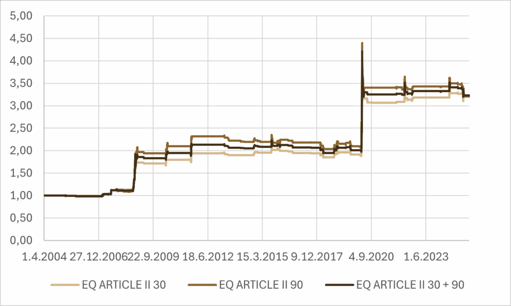
Table 7: Performance metrics of modified article strategies using sizing and their composition.
| PORTFOLIO | CAR p.a. | VOL p.a. | SHARPE |
|---|---|---|---|
| 10D SD & 30D MA for VIX strategy | 6.55% | 11.91% | 0.30 |
| 10D SD & 90D MA for VIX strategy | 7.18% | 12.85% | 0.56 | Composition of 30D and 90D strategy | 6.90% | 12.14% | 0.57 |
When we combine the 30-day and 90-day VIX-based strategies into a single composite approach, we observe a marginal improvement in risk-adjusted performance compared to the individual strategies. While each of the original strategies performs reasonably well on its own, the composite slightly enhances the Sharpe ratio, suggesting that blending different horizons can modestly smooth returns and mildly improve efficiency without drastically changing the overall risk profile.
As the final step of this analysis, we need to address combinations of these strategies with SPY. By allocating 80% of the portfolio to SPY and the remaining portion to the strategies described above, sometimes using leverage, we obtain the following results.
* In benchmark strategy, between 01.04.2004 and 03.12.2007, 20% of portfolio was in cash.
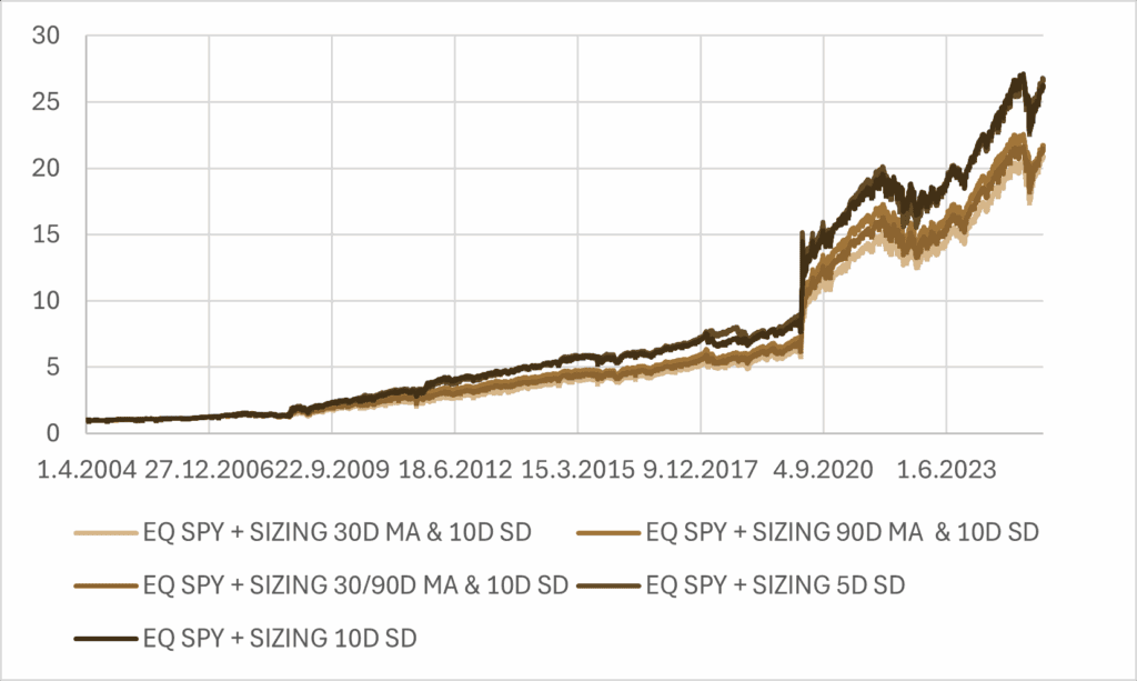
Table 8: Performance metrics of benchmark and modified article strategies using sizing and their composition and modified article strategies not using sizing or smoothing.
| PORTFOLIO | CAR p.a. | VOL p.a. | SHARPE |
|---|---|---|---|
| 100% SPY | 10.52% | 18.71% | 0.56 |
| 80% SPY, 20% VXV-VIX signal strategy (benchmark) | 6.25% | 16.29% | 0.38 |
| 80% SPY + SIZING 30D MA & 10D SD (eVRP) strategy | 16.47% | 15.76% | 1.04 |
| 80% SPY + SIZING 90D MA & 10D SD (eVRP) strategy | 17.38% | 15.44% | 1.13 |
| 80% SPY + SIZING 30D/90D MA & 10D (eVRP) strategy | 16.96% | 15.41% | 1.10 |
| 80% SPY + 5D (eVRP) strategy | 11.00% | 13.72% | 0.80 | 80% SPY + 10D (eVRP) strategy | 10.91% | 13.59% | 0.8 | 80% SPY + SIZING 5D (eVRP) strategy | 18.39% | 15.52% | 1.19 | 80% SPY + SIZING 10D (eVRP) strategy | 18.17% | 15.32% | 1.19 |
When combining SPY with the strategies derived above, we can clearly see that not all approaches add value. The simple benchmark combination with the VXV–VIX signal actually dilutes performance relative to holding SPY alone, both in terms of absolute and risk-adjusted returns.
By contrast, strategies that incorporate dynamic sizing deliver much more attractive outcomes. Whether sizing is based on the 30-day or 90-day moving average, or a composite of the two, the improvements are evident. These approaches simultaneously increase returns and reduce risk compared to SPY on its own, resulting in a substantial boost in efficiency.
Even the simpler 5-day and 10-day eVRP variants provide some benefit, though their impact is less pronounced. Once dynamic sizing is added to these shorter windows, however, the performance becomes particularly compelling, combining higher returns with improved stability.
Conclusion
Our analysis shows that tail-hedging strategies based on eVRP signals can provide meaningful improvements when carefully designed and implemented. While naive benchmarks or unsized variants often fail to outperform a simple SPY allocation, introducing position sizing linked to VIX levels consistently enhances both returns and risk-adjusted outcomes. Among the variations considered, dynamically sized strategies, whether based on short or medium-term windows, stand out as the most effective complements to a core SPY portfolio.
An important outcome of this analysis is that the introduction of sizing allowed us to identify several relatively efficient strategies. What also becomes clear is that the hedge activates only rarely within the portfolio. Yet when it does, and when the conditions are properly defined, the results can be quite compelling. This highlights the value of having a well-calibrated hedging mechanism in place: it does not burden the portfolio during normal market conditions, but it can meaningfully improve outcomes when stress events occur.
Authors:
David Belobrad, Junior Quant Analyst, Quantpedia
Radovan Vojtko, Head of Research, Quantpedia
Are you looking for more strategies to read about? Sign up for our newsletter or visit our Blog or Screener.
Do you want to learn more about Quantpedia Premium service? Check how Quantpedia works, our mission and Premium pricing offer.
Do you want to learn more about Quantpedia Pro service? Check its description, watch videos, review reporting capabilities and visit our pricing offer.
Do you want algorithmic access to the full Quantpedia database via the API? Subscribe to Quantpedia Pro, ask for an API key, and explore the in/out-of-sample statistics, source academic papers, and code snippets — ideal for quantitative research, systematic trading workflows, and AI model training.
Are you looking for historical data or backtesting platforms? Check our list of Algo Trading Discounts.
Or follow us on:
Facebook Group, Facebook Page, Telegram, Twitter, Linkedin, Medium or Youtube
Share onLinkedInTwitterFacebookRefer to a friend


