Niels Bohr, the Nobel laureate in Physics, famously said, “Prediction is very difficult, especially if it’s about the future.”. In the domain of financial analysis, estimating the long-run returns of equities over a horizon of 10 to 20 years presents a formidable challenge. Despite the significant challenges in accurately forecasting market trends and economic conditions over such lengthy periods, this task remains important for investors, portfolio managers, and policymakers, as some of them often depend on these forecasts to develop effective investment strategies and policy frameworks. Input from today’s reviewed paper provides valuable insights on how to improve these predictions.

The paper straightforwardly named Estimating Long-Term Expected Returns deals with accurately estimating long-term expected returns of equity markets, which is essential for corporate entities and individual investors in the same way. They investigate the ability of different frameworks and input proxies to estimate 10- and 20-year OOS returns over long historical time periods and more recent periods. They found that several approaches generate meaningful improvements compared to historical mean model forecasts. OOS-R2 can be as significant as 40% even in the most recent period, and asset allocation based on presented model forecasts can improve a portfolio’s Sharpe ratio and VaR by over 50%.

The methodologies authors undertook consist of running various frameworks and proxies used to generate long-term E(R) forecasts and comparing the approaches’ performance to estimate expected returns that have primarily been considered in isolation. They show that 10- to 20-year E(R)s can be estimated ex-ante: Out-of-sample (OOS) forecast improvements over historical mean forecasts are as large as 40% even in the most recent period. Importantly, these gains exist within a range of time periods.

Results are of interest to those who require accurate long-term expected return forecasts, and we especially encourage avid readers to look at Tables 1 and 2, which provide insightful summaries of critical findings in the paper.

Authors: Rui Ma, Ben R. Marshall, Nhut H. Nguyen, Nuttawat Visaltanachoti

Title: Estimating Long-Term Expected Returns

Link: https://papers.ssrn.com/sol3/papers.cfm?abstract_id=4493448

Abstract:

Estimating long-term expected returns as accurately as possible is of critical importance. Researchers typically base their estimates on yield and growth, valuation, or a combined yield, growth, and valuation framework. We run a horse race of the abilities of different frameworks and input proxies within each framework to estimate 10- and 20-year out-of-sample returns over 140-year and more recent time periods. Our results indicate that several approaches strongly outperform estimates based on historical mean benchmark returns, with mean square error improvements exceeding 40%. Using these approaches in asset allocation decisions results in an improvement in Sharpe ratios of more than 50%.

As always we present several interesting figures and tables:

Notable quotations from the academic research paper:

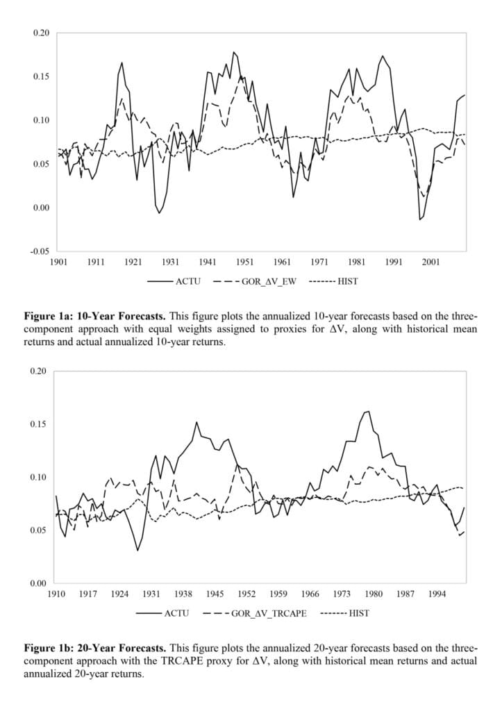
“Our results indicate that the three-component framework is superior for 10-year forecasts, although not by a large margin. The three-component model that generates ΔV estimates based on the wealth portfolio composition of Rintamaki (2023), denoted as VWPC, outperforms other three-component models in forecasting 10-year returns for the entire sample period from 1891 to 2020. However, in two more-recent sub-sample periods, it is not statistically different from other three-component models, such as the one that assigns an equal weight to four proxies for ΔV. We suggest that this latter model is superior overall, as it performs better in an asset allocation setting. It generates a 34.91% reduction in MAEs and a 57.70% increase in OOS-R2 compared to the historical mean model for 10-year forecasts over the 1891–2020 sample period. Furthermore, a stock-bond portfolio with weights allocated based on these E(R) forecasts has an approximately 65.56% higher Sharpe ratio and a 50.06% improvement in value at risk (VaR) over the 1891–2020 period. Importantly, this model also leads to improvement gains in more recent periods. Twenty-year returns are typically more difficult to forecast. However, several approaches, such as the three-component model with the total return cyclically adjusted price-to-earnings ratio (TRCAPE) proxy significantly enhance the accuracy of these predictions.

We contribute to several strands of the long-term return predictability literature. Fama and French (1988) use a yield-alone approach and show that dividend yields explain more han 25% of the variance of two- to four-year returns. Campbell and Shiller (1998) contribute to the valuation-alone literature by focusing on predicting 10-year returns using a price-to- earnings ratio that is derived from the average earnings over the last 10 years. They suggest that accounting for earnings fluctuations over the business cycle is important and show that this metric, which is widely referred to as the cyclically adjusted price-to-earnings ratio (CAPE), is effective at predicting stock returns. Bogle (1991a, b) introduces the three- component approach and suggests that the forecasts of the 10-year returns give “a remarkably precise replication of the actual total returns realized.”

We present summary statistics in Table 1. The average annual returns are 10.66%, 11.76%, and 12.27% for the 1872–2020, 1955–2020, and 1988–2020 periods, respectively. Returns have negative skewness across all three sample periods. Kurtosis is negative for the entire period, but positive in the more recent periods. In Panel B, we present mean geometric and log returns for 10-year and 20-year intervals rolling forward one year at a time. It is these annualized log returns that we use in our model forecasts. For the 10-year interval, average annualized log returns are 8.65%, 9.40%, and 8.57% for the three periods, respectively, while for the 20-year interval, these are 8.73%, 9.68%, and 7.55%, respectively. Similarly, Panel C reports the standard deviation of geometric returns and log returns for 10-year and 20-year intervals rolling forward one year at a time.

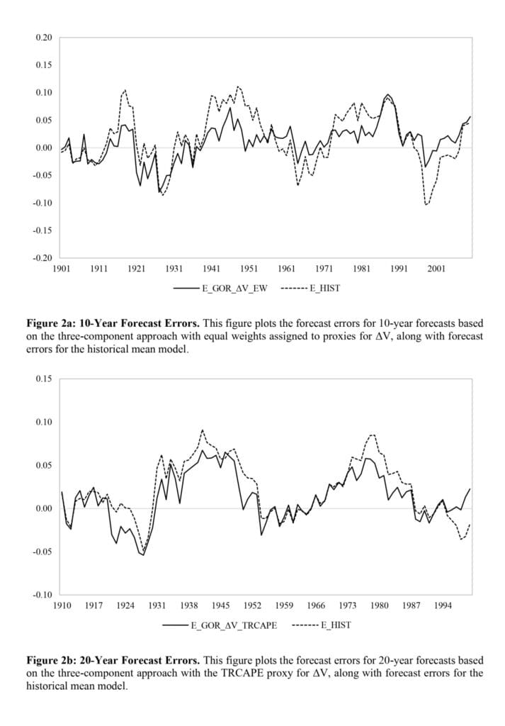
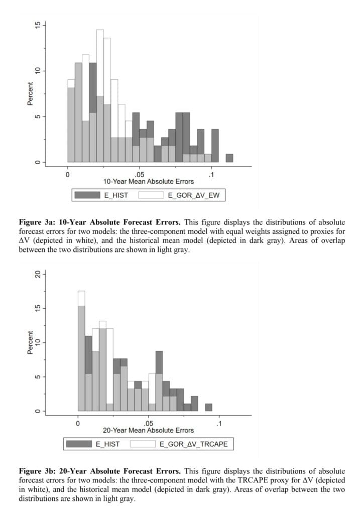
In Table 2, we report results for 10-year forecasts. We calculate the MAE as the average absolute difference between the forecast and actual returns. We also calculate the difference in MAEs between each prediction model and the historical mean forecast.⁷ We measure the statistical significance of this difference using the moving block bootstrap method, which accounts for autocorrelation in the time series. The optimal block length is determined as per Patton, Politis, and White (2009). For each prediction model, we generate 1000 bootstrap resamples and report statistical significance based on the one-sided bootstrap p-value (i.e., the proportion of the bootstrap sample prediction model MAEs that exceed the historical mean model MAE in the same bootstrap sample).

The results in Table 2 indicate that the three-component framework is the best- performing framework. For 10-year forecasts, this framework has the lowest average MAE in the 1981–2020, 1955–2020, and 1988–2020 periods. To ascertain the statistical difference between the “three components” framework and the other three frameworks (i.e., “yield alone,” “Gordon,” and “valuation alone”), we first compute the yearly average absolute error for each framework over time. Utilizing the resulting four time series, we then apply the Diebold–Mariano test (Diebold and Mariano, 1995). As shown in Appendix 3, the average absolute error of “three components” is statistically significantly lower than “Gordon” in all three time periods and statistically significantly lower than “valuation alone” and “yield alone” in two of the three time periods.”

Are you looking for more strategies to read about? Sign up for our newsletter or visit our Blog or Screener.

Do you have an idea for systematic/quantitative trading or investment strategy? Then join Quantpedia Awards 2024!

Do you want to learn more about Quantpedia Premium service? Check how Quantpedia works, our mission and Premium pricing offer.

Do you want to learn more about Quantpedia Pro service? Check its description, watch videos, review reporting capabilities and visit our pricing offer.

Are you looking for historical data or backtesting platforms? Check our list of Algo Trading Discounts.

Or follow us on:

Facebook Group, Facebook Page, Twitter, Linkedin, Medium or Youtube