Introduction to Clustering Methods In Portfolio Management – Part 3
This is the third and final article from the clustering series. If you’ve missed the previous parts, here you can find the first and second parts of the series. This section examines trading strategies based on previously introduced clustering methods. The complete Portfolio Clustering report will be available for our Quantpedia Pro clients next week.
Cluster Risk Parity Strategies
In one of the blogs, we introduced Risk Parity Asset Allocation as a portfolio management methodology that focuses on risk allocation (how to find weights of assets that ensure an equal level of risk, most frequently measured by the volatility). However, as mentioned in the first part of this series, it does not take into consideration a type of asset class and the number of assets in each asset class.
Therefore, even though using pure risk parity can be helpful in many cases, it can undoubtedly be improved. In this section, we will build six investment strategies based on clustering our 8 ETFs, including four equities (SPY–SPDR S&P 500 ETF Trust, VGK–Vanguard FTSE Europe Index Fund ETF Shares, EEM–iShares MSCI Emerging Markets ETF, VPL–Vanguard FTSE Pacific Index Fund ETF Shares), two alternatives (DBC–Invesco DB Commodity Index Tracking Fund, GLD–SPDR Gold Shares) and two bond ETFs (IEF–iShares 7-10 Year Treasury Bond, BNDX–Vanguard Total International Bond Index Fund ETF Shares).
The first three strategies will firstly create optimal clusters and then weigh assets inside the clusters equally and clusters among themselves equally as well (Clustering Equal Weight). The second three strategies will do the same, but instead of using equal intra-cluster and inter-cluster weights, they will weigh the assets inside the cluster and the clusters between themselves proportionately to the inverse of their volatility, i.e. according to Naïve risk parity (Cluster Risk Parity).
For each of the two weighing schemes mentioned above, we will be analyzing 3 different clustering methods – PAM, AGNES and GMM – arriving to 2 * 3 = 6 strategies.
Methodology
Firstly, we sort the assets into clusters on a weekly frequency. We use the same eight assets as in the previous section. We use data from 20/05/2014 to 24/05/2021, and each week we sort them into clusters based on past one-year weekly returns. As mentioned, we use three clustering methods: Partitioning Around Medoids (PAM), Hierarchical clustering (AGNES), specifically agglomerative average linkage and lastly, Gaussian Mixture Model (GMM). The optimal number of clusters is determined using the silhouette method.
Results
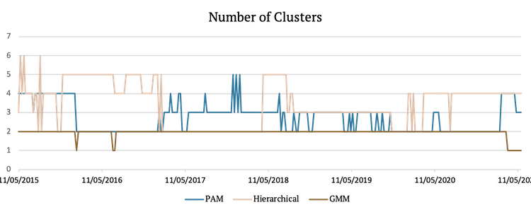
The following figure shows the optimal number of clusters chosen using the silhouette method at each point in time for each method. As we can see, GMM almost always picks two clusters and also chooses the lowest number of clusters out of all methods. Hierarchical clustering picks between two and six clusters, and PAM selects from two to five clusters depending on the period.
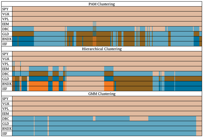
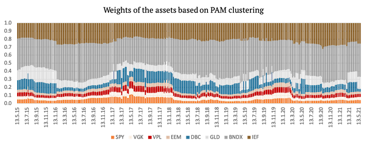
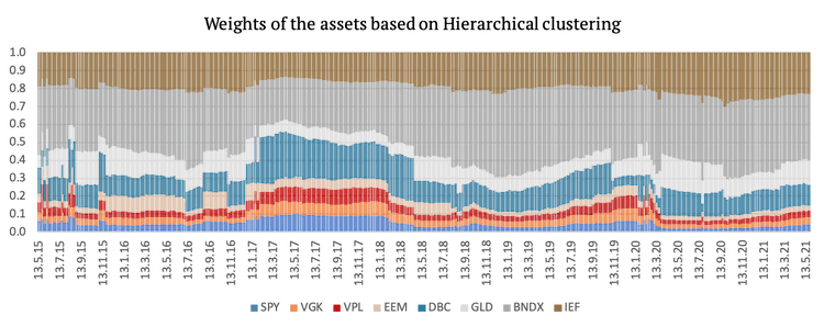
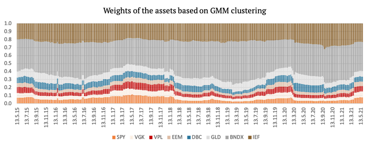
The following chart graphically represents how each clustering method sorted the assets at every point in time. Each color represents one cluster, meaning that assets with the same color belong to the same cluster.
Clustering Strategies
Now that we sorted the assets into clusters, we can create the six aforementioned strategies. The first three strategies give equal weights to the clusters and also equal weights to assets within clusters (Equal weights between clusters and within clusters). The second three strategies give weights to the clusters so that their volatility contribution is equal; the same is done to the assets within clusters (Naïve Risk Parity between clusters and within clusters).
We will benchmark the first three strategies against an equal weight portfolio of 8 ETFs. We will benchmark the second three strategies against the standard Naïve Risk Parity portfolio of 8 ETFs.
Equal Cluster Weights
The following figure shows the cumulative returns of the first three strategies based on the three clustering methods and the cumulative return of the benchmark (equally-weighted) portfolio.
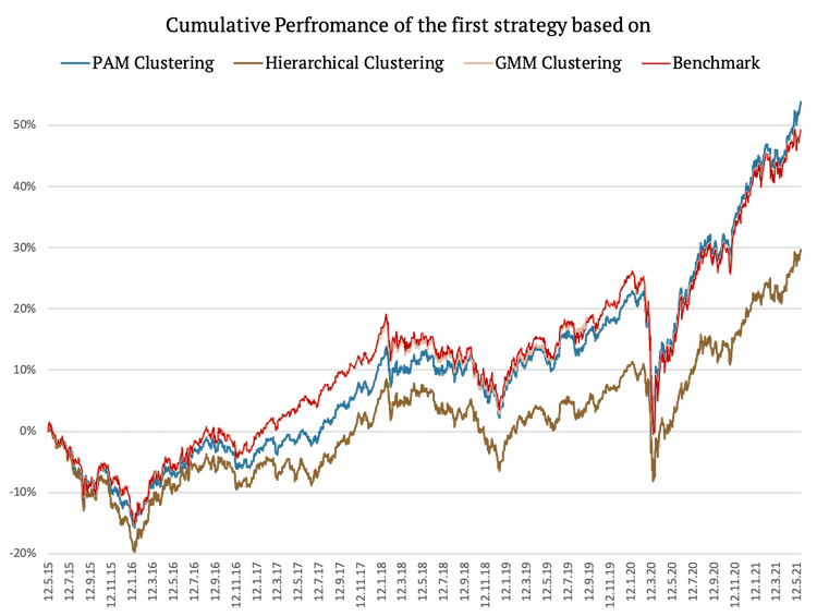
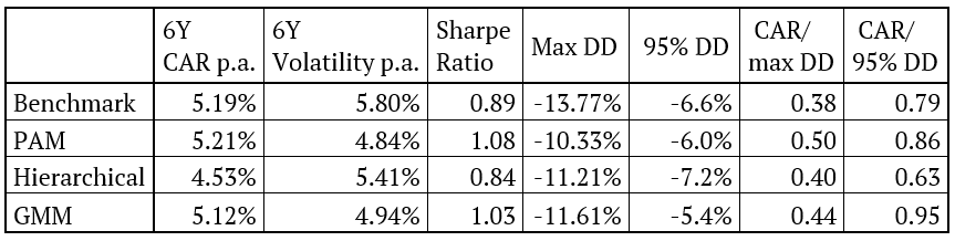
As we can see, a strategy which assigns equal weights to assets and clusters based on PAM clustering achieved the best risk-adjusted performance. Hierarchical clustering underperformed, mainly due to giving a bigger weight to commodities (which underperformed in the period under review). Additionally, the performance of the benchmark portfolio is very similar to the performance of the strategy based on GMM clustering. This is caused by the fact that GMM chose two clusters, both including four assets, for most of the periods, thus arriving to identical weights to the equal weight benchmark. The table below presents the risk and return characteristics of all three strategies plus the benchmark.
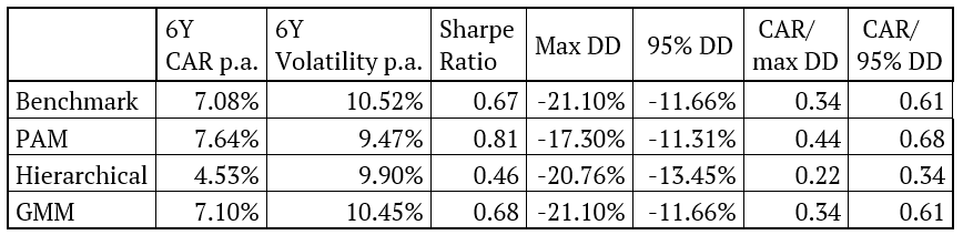
As we can see, the 6-year CAR of the strategy based on GMM is closest to the benchmark. However, the strategy based on PAM clustering performed best with the highest Sharpe ratio of 0.81 and smallest drawdown of -17.30%.
Lastly, we present a graphical representation of the weights of the assets used in the first three strategies.
Cluster Risk Parity
Now let’s look at the second three strategies (Naïve Risk Parity between clusters and within clusters) and their cumulative performances.
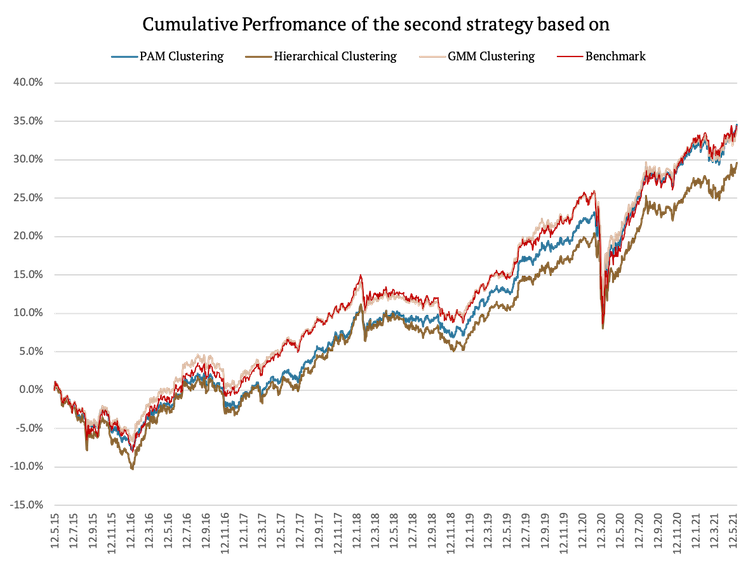
As was the case with the first three strategies, PAM clustering which assigns risk parity weights to assets and clusters achieved the best risk-adjusted performance. Hierarchical clustering again underperformed, mainly due to giving again a bigger weight to commodities (which underperformed in the period under review). In this case even GMM outperformed the benchmark on a risk-adjusted basis. Moreover, Sharpe ratios of all strategies using Naïve Risk Parity improved significantly.
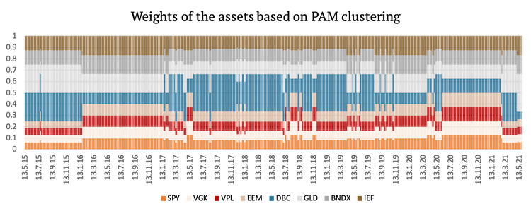
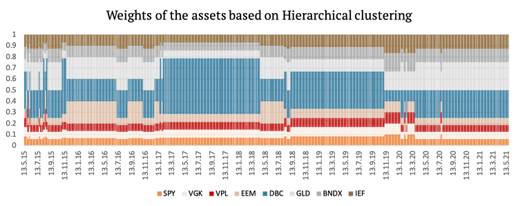
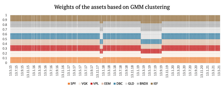
Lastly, we present a graphical representation of the weights of the assets used in the second three strategies. The weights change more frequently in this case because even if the clusters remain the same, the volatility of the assets is always changing.
Conclusion
What can we take out of this quick example?
Firstly, naturally, it makes sense to combine the clustering method with risk parity weighting. That’s the point of doing clustering analysis; it doesn’t make sense to use equal weighting inside clusters or among clusters, as our goal is to weight clusters according to their risk.
Secondly, the clustering algorithm is not a cure-all method. It doesn’t always increase the performance or Sharpe ratio of the resulting portfolio. Sometimes, clustering can increase the weight of an asset that underperforms. But clustering should not be used to identify outperforming assets but for risk management. It’s a very useful method to estimate how many assets/strategies that are similar we have in our portfolio so that we can better diversify among them. But clustering algorithms need to be used with a return predictor (for example, momentum) to select assets we want to have in the portfolio.
Author:
Daniela Hanicova, Quant Analyst, Quantpedia
Are you looking for more strategies to read about? Sign up for our newsletter or visit our Blog or Screener.
Do you want to learn more about Quantpedia Premium service? Check how Quantpedia works, our mission and Premium pricing offer.
Do you want to learn more about Quantpedia Pro service? Check its description, watch videos, review reporting capabilities and visit our pricing offer.
Do you want algorithmic access to the full Quantpedia database via the API? Subscribe to Quantpedia Pro, ask for an API key, and explore the in/out-of-sample statistics, source academic papers, and code snippets — ideal for quantitative research, systematic trading workflows, and AI model training.
Are you looking for historical data or backtesting platforms? Check our list of Algo Trading Discounts.
Or follow us on:
Facebook Group, Facebook Page, Telegram, Twitter, Linkedin, Medium or Youtube
Share onLinkedInTwitterFacebookRefer to a friend


