Leveraged ETFs in Asset Allocation: Opportunity or Trap?
In this article, we explore whether it makes sense to incorporate leveraged ETFs into static and dynamic long-only asset allocation strategies. Leveraged ETFs promise amplified exposure to the underlying asset, offering the potential for significantly higher returns during favorable market conditions. However, this comes at the cost of much higher volatility, path-dependency, and the well-known issue of volatility decay, which can lead to substantial underperformance over longer periods. Our objective is to examine if — and how — leveraged ETFs can be systematically integrated into portfolio construction so that their benefits can be captured while mitigating their inherent risks.
Part I
Introduction
Leveraged Exchange-Traded Funds (LETFs) are a highly debated topic in the financial literature. These funds aim to deliver a multiple (typically two or three times) of the daily return of an underlying benchmark index. Due to their ability to amplify market exposure, they quickly gained popularity among retail investors, institutional investors (DeVault et al., 2021[1]), and short-term traders. However, research consistently highlights that LETFs are not intended for long-term buy-and-hold strategies (Avellaneda & Zhang, 2010[2]; Lu, Wang, & Zhang, 2009[3]; Charupat & Miu, 2011[4]). The main concern centers on the compounding effect: because a leveraged ETF multiplies daily returns, it does not achieve the same multiple over longer horizons. As a result, extended holding periods can lead to performance erosion and potential losses. While these criticisms of leveraged ETFs are valid, recent research suggests that their potential benefits may have been underestimated (Van Staden, Forsyth, and Li, 2024[5]). Building on this perspective, the goal of our research is to find out whether leveraged ETFs can improve portfolio performance compared to traditional benchmarks.
Data & Methodology
Our investment universe spans from 1926 to 2025 and includes monthly data for both leveraged and non-leveraged versions of four main asset classes ETFs, as well as cash.
We used daily data for U.S. equities (SPY), commodities (USO), U.S. 10-year Treasuries (IEF), and gold (GLD). To construct proxy double-leveraged ETFs, we simulated 2× leverage by doubling the daily returns of each asset class and then subtracting daily management fees and leverage costs.
When actual double-leveraged ETFs became available, their historical data were incorporated into the dataset to replace the simulated values for the corresponding periods. These include SSO (2× S&P 500, 2006), UCO (2× oil, 2023), UST (2× Treasuries, 2010), and UGL (2× gold, 2008).
We began by analyzing passive portfolios composed of individual asset classes. The performance and risk characteristics of each non-leveraged ETF are shown in Table 1, and those for leveraged ETFs in Table 2.
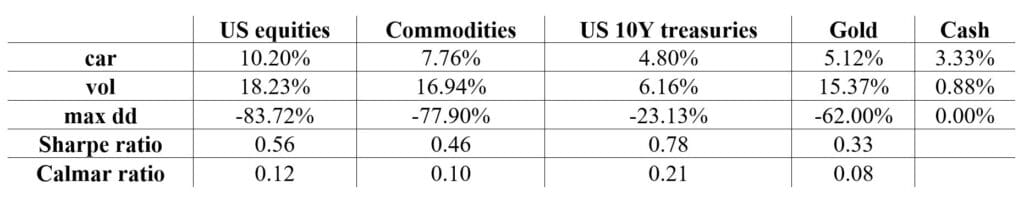
Table 1. Performance and risk characteristics of each asset class ETF
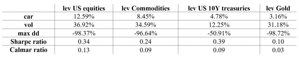
Table 2. Performance and risk characteristics of each asset class leveraged ETF
Result 1
Leveraging bonds and gold ETFs mostly increases risk while lowering returns. For example, the U.S. 10-year Treasury ETF sees its volatility rise from 6.16% to 12.25%, while its annual return slightly decreases from 4.80% to 4.78%. For commodities, performance improves slightly, but volatility more than doubles. Leveraging equities increases both risk and return (car from 10.20% to 12.59%, vol from 18.23% to 36.92%), suggesting that leverage can improve portfolio performance if used strategically.
The data from Table 1 and Table 2 are illustrated in Graphs 1–4, which show the equity curves of different assets and their leveraged versions over the past 100 years, plotted on a logarithmic scale.
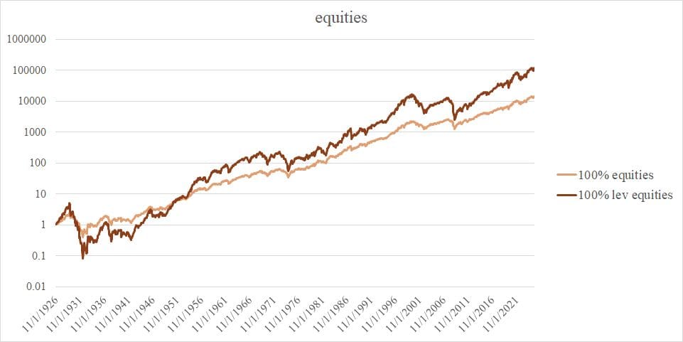
Graph 1. Equity curves of U.S. equities and leveraged U.S. equities
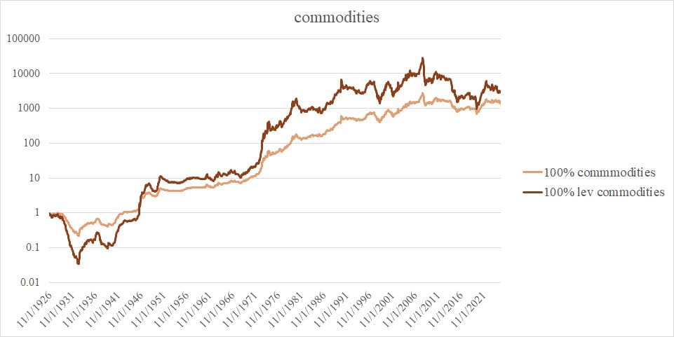
Graph 2. Equity curves of commodities and leveraged commodities
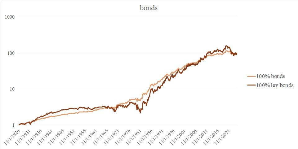
Graph 3. Equity curves of U.S. 10-year treasuries and leveraged treasuries
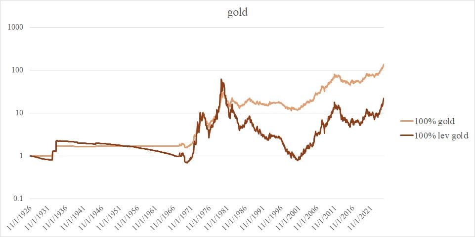
Graph 4. Equity curves of gold and leveraged gold
Our next step was to apply Markowitz portfolio optimization to test whether incorporating leveraged ETFs could improve overall portfolio performance. Specifically, we tested whether even a small allocation to leveraged equities could improve the risk–return profile and whether introducing leverage would shift the efficient frontier.
We constructed two sets of portfolios as inputs for the optimization:
- a 60/40 portfolio consisting of equities and bonds, and the same portfolio where equities were replaced with leveraged equities, and
- a portfolio consisting of 25% equities, 10% gold, and 65% bonds, along with its version using leveraged equities instead of standard equities.
We focused only on leveraged SPY, since, as shown in Table 1, equities showed the greatest potential for improving performance relative to other asset classes. The optimization was conducted using Quantpedia Pro Portfolio Analysis.
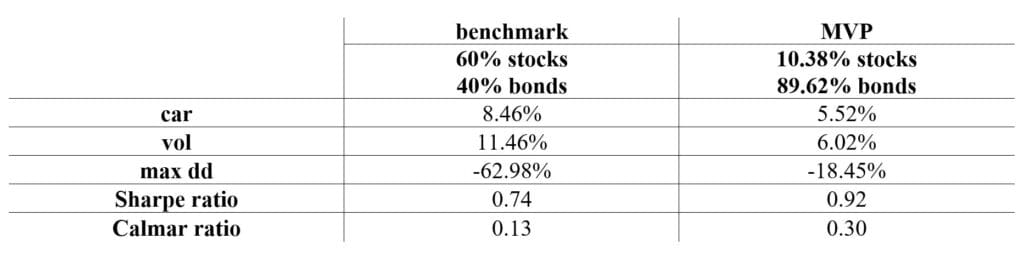
Table 3. Performance and risk characteristics of 60/40 benchmark and Markowitz minimum variance portfolio
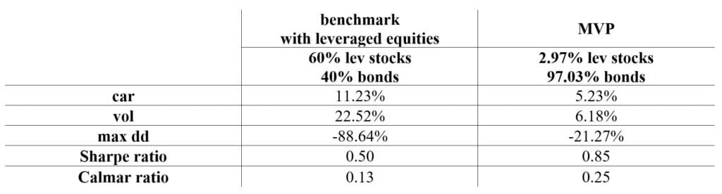
Table 4. Performance and risk characteristics of 60/40 benchmark with leveraged equities and Markowitz minimum variance portfolio with leveraged equities
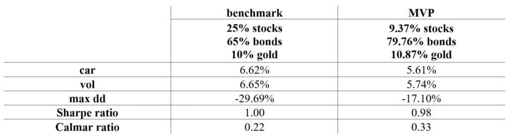
Table 5. Performance and risk characteristics of 25/65/10 benchmark and Markowitz minimum variance portfolio
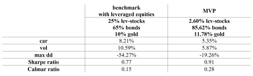
Table 6. Performance and risk characteristics of 25/65/10 benchmark with leveraged equities and Markowitz minimum variance portfolio with leveraged equities
Result 2
As Tables 3-6 show, the minimum variance portfolio is dominated by bonds. When leveraged equities are added (tables 4 & 6), their weight in the portfolio is minimized compared to the non-levered portfolios (table 3 & 5). Even so, even then overall risk is higher and returns are lower compared to non-leveraged portfolios. Across all benchmark comparisons, replacing equities with leveraged equities worsened portfolio performance.
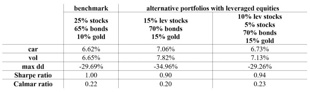
Table 7. Performance and risk characteristics of 25/65/10 benchmark and alternative portfolios with leveraged equities
In addition, we tested alternative allocations where the share of leveraged equities equals their non-leveraged equivalents (for example, 10% in leveraged equities = 20% in regular equities). Our hope was that by shifting allocation to levered ETFs, we would save money/cash and could invest in more assets (for example, add bonds). As shown in Table 7, these portfolios do not outperform the benchmark once risk is considered.
We conclude that leveraged ETFs do not work well for long-term passive investing. Leverage increases both gains and losses, and over time this leads to weaker overall performance.
Part II:
The first part of our research, focused on the use of leveraged ETFs to improve portfolio performance, concluded that leveraged ETFs perform poorly in long-term passive portfolios. Although leveraged equity ETFs showed some potential, they did not improve the risk–return characteristics of a passive strategy. In this second part, we explore whether leverage can become beneficial when actively managed, specifically when combined with a trend-following strategy.
Methodology
We focused on two trend-following models: i) 10-Month Moving Average rule (Faber, 2007): if the end-of-month price of an asset is above its 10-month moving average, the strategy takes a position in the asset for the next month; otherwise, it moves to cash. ii) 95 – 100% of 12-Month High rule (Faber, 2025): if the end-of-month price is within 95 – 100% of its 12-month high, the strategy takes a position in the asset for the next month; otherwise, it moves to cash.
We applied the 10-Month Moving Average model to 4 asset classes: U.S. equities (SPY), commodities (USO), U.S. 10-year Treasuries (IEF), and gold (GLD). We first calculated the indicator (the moving average) and then set a simple monthly signal (either buy the asset or hold cash in the following month). Performance of this strategy for each asset class is summarized in Table 8. We then repeated the same procedure for the leveraged versions of these assets (2× SPY, 2× USO, 2× IEF, and 2× GLD) and the results are summarized in Table 9.
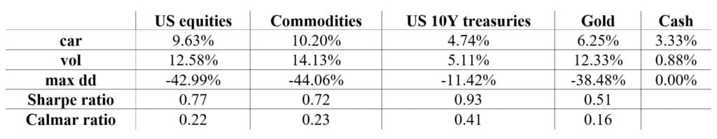
Table 8. Performance and risk characteristics: 10-Month Moving Average rule
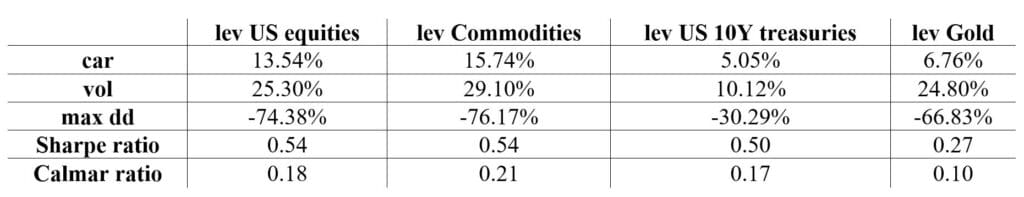
Table 9. Performance and risk characteristics: 10-Month Moving Average rule, leveraged ETFs
Result 3a
When comparing the results of the trend filter applied to non-leveraged ETFs (Table 8) with the benchmark (Table 1), we find that the trend filter improves the risk–return profile. The overall risk decreases (vol from 18.23% to 12.58% for equity ETF), so does the return (car from 10.20% to 9.63% for equity ETF). When applying the same trend filter to leveraged ETFs (Table 9), both risk and performance increase (vol from 18.23% to 25.30%, car from 10.20% to 13.54% for equity ETF).
Similarly, we applied the 12-Month High Rule to both non-leveraged and leveraged versions of the same assets. We first calculated the indicator (the highest price within the last 12 months) and then generated a simple monthly signal (buy the asset or hold cash). The performance of this strategy is summarized in Table 10 for non-leveraged ETFs and Table 11 for leveraged ETFs.
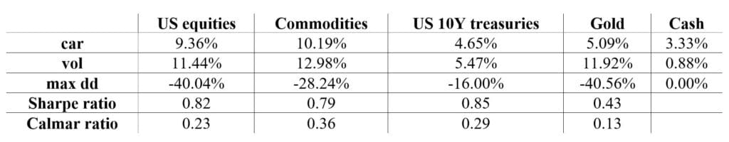
Table 10. Performance and risk characteristics: 12-Month High rule
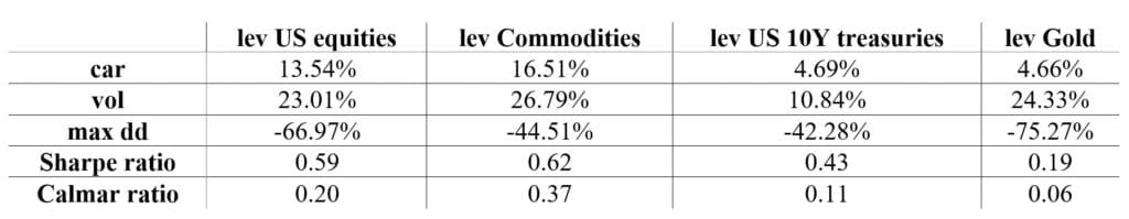
Table 11. Performance and risk characteristics: 12-Month High rule, leveraged ETFs
Result 3b
The results for the 12-Month High model are consistent with those of the 10-Month Moving Average model. The trend filter improves the risk–return ratio for non-leveraged ETFs (Table 10), lowering both risk (vol from 18.23% to 11.44% for equity ETF) and performance (car from 10.20% to 9.36% for equity ETF). For leveraged ETFs (Table 11), the trend filter increases both risk (vol from 18.23% to 23.01% for equity ETF) and performance (car from 10.20% to 13.54% for equity ETF).
Overall, the trend filters improve the risk–return profile of non-leveraged ETFs, while for leveraged ETFs, both risk and return rise, and the Sharpe and Calmar ratios remain similar or slightly improved compared to passive benchmark.
In the next step, we test portfolios that include trend-filtered leveraged equity ETFs to see whether these active strategies can further improve overall performance.
Our conservative benchmark (Portfolio 1) consists of 25% equities, 65% bonds, and 10% gold ETFs.
Portfolio 2 has the same allocation but applies a trend-following filter (10-month moving average) to all assets. The trend-based portfolio shows lower risk but also slightly lower performance, in accordance with previous section. Our goal is to find a portfolio that keeps the lower risk of the trend-based strategy while improving returns. To achieve this, we include leveraged equity ETFs. We do not leverage bonds or gold, as this would increase overall portfolio risk. We therefore construct Portfolio 3, a trend-following portfolio with a share of leveraged equities. It gradually replaces part of the regular equity position with leveraged equities. Our final portfolio consists of 5% equities, 10% gold, 65% bonds, 20% leveraged equities ETFs. The performance and risk metrics are shown in Table 12.
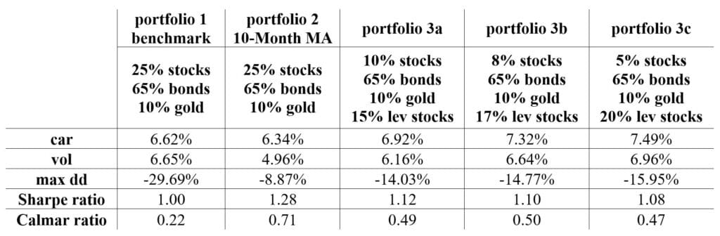
Table 12. Performance and risk characteristics: 25/65/10 portfolio
Result 4
Portfolio 3 achieves higher performance while maintaining volatility comparable to the benchmark. The performance and risk dynamics of the these two portfolios are shown in Graph 5 (equity curve) and Graph 6 (drawdown). These results suggests that introducing a share of leveraged equities within an active trend-based strategy can improve returns without disproportionally increasing risk!
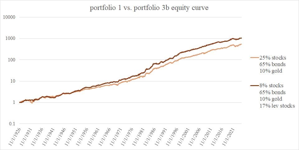
Graph 5. Equity curves of portfolio 1 (25% stocks, 65% bonds, 10% gold) and portfolio 3b (8% stocks, 65% bonds, 10% gold, 17% lev stocks)
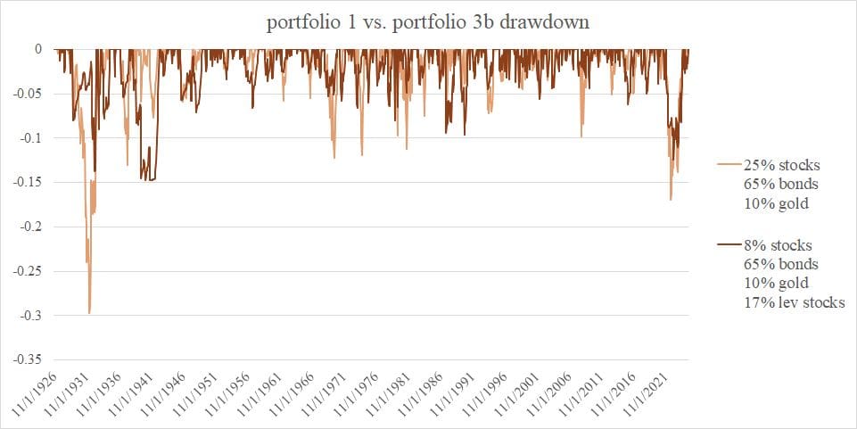
Graph 6. Drawdown of portfolio 1 (25% stocks, 65% bonds, 10% gold) and portfolio 3b (8% stocks, 65% bonds, 10% gold, 17% lev stocks)
Building on 60/40 equity-bond portfolio, our Portfolio 1 consists of 60% equities and 40% bonds. We improve the risk-return characteristics by introducing gold, creating a Portfolio 2 with 50% equities, 40% bonds, 10% gold ETFs. Applying a trend following filter (Portfolio 3) to this allocation reduces volatility, improves both Sharpe and Calmar rations, though at the cost of lower returns. To boost the performance, we introduce leveraged equities. In Portfolio 4, 30% of the non-leveraged equity exposure is replaced with leveraged equities, creating a portfolio of 20% equities, 40% bonds, 10% gold, 30% leveraged equities ETFs. The performance and risk metrics are shown in Table 13.
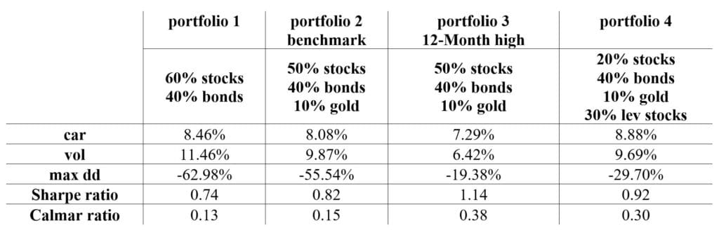
Table 13. Performance and risk characteristics: 60/40 portfolio
Result 5
The 20% equities, 40% bonds, 10% gold, 30% leveraged equities ETFs portfolio keeps risk at a similar level to Portfolio 2 while improving performance. The performance and risk dynamics of portfolio 1 and 4 are shown in Graph 7 (equity curve) and Graph 8 (drawdown).
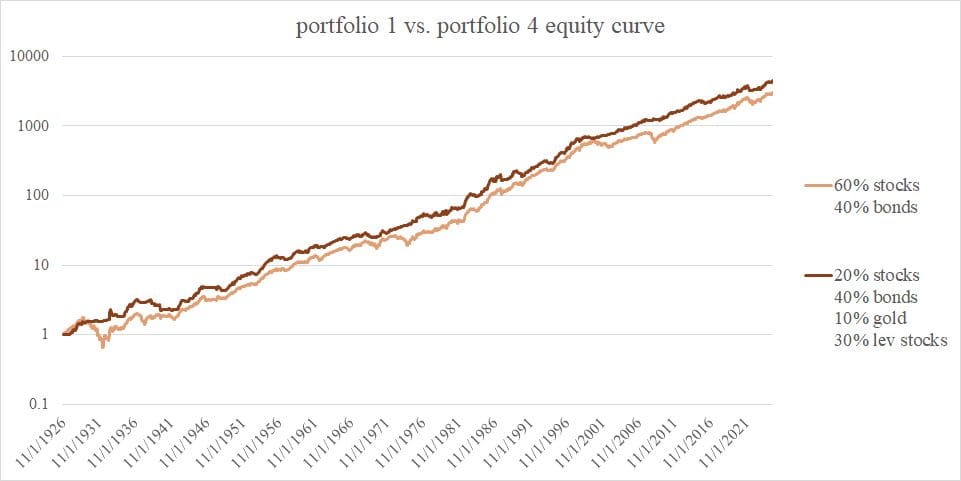
Graph 7. Equity curves of portfolio 1 (60% stocks, 40% bonds) and portfolio 4 20% stocks, 40% bonds, 10% gold, 30% lev stocks)
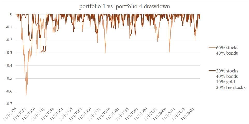
Graph 8. Drawdown of portfolio 1 (60% stocks, 40% bonds) and portfolio 4 20% stocks, 40% bonds, 10% gold, 30% lev stocks)
In both portfolios, trend-following strategies helped reduce risk and drawdowns, but also slightly lowered returns. When we added a small share of leveraged equities to these trend-based portfolios, performance improved while risk stayed under control, comparable to the benchmark. This shows that leverage can be beneficial only when it is actively managed.
Conclusion
Our study tested whether leveraged ETFs can improve portfolio outcomes relative to standard benchmarks.
Part I showed that leveraged ETFs do not work well in long-term passive portfolios. While they amplify returns, they also amplify losses and volatility. The Markowitz optimization confirmed that replacing equities with leveraged equities does not improve results. Portfolios with leveraged ETFs stay dominated by bonds, and their risk–return ratios are worse than those of non-leveraged portfolios.
Part II tested whether leverage can be useful when actively managed. Using two simple trend-following models (10-month moving average and 12-month high), we found that trend filters reduce risk and drawdowns for non-leveraged assets but also lower returns. For leveraged assets, both risk and returns increase.
Overall, the results show that leveraged ETFs only make sense when risk is actively managed. They perform poorly as passive investments, but when used carefully within a trend-following strategy, they can improve returns without a large increase in risk
Author: Margareta Pauchlyova, Quant Analyst, Quantpedia
Are you looking for more strategies to read about? Sign up for our newsletter or visit our Blog or Screener.
Do you want to learn more about Quantpedia Premium service? Check how Quantpedia works, our mission and Premium pricing offer.
Do you want to learn more about Quantpedia Pro service? Check its description, watch videos, review reporting capabilities and visit our pricing offer.
Do you want algorithmic access to the full Quantpedia database via the API? Subscribe to Quantpedia Pro, ask for an API key, and explore the in/out-of-sample statistics, source academic papers, and code snippets — ideal for quantitative research, systematic trading workflows, and AI model training.
Are you looking for historical data or backtesting platforms? Check our list of Algo Trading Discounts.
Or follow us on:
Facebook Group, Facebook Page, Telegram, Twitter, Linkedin, Medium or Youtube
Literature:
[1] DeVault, L., Turtle, H. J., & Wang, K. (2021). Blessing or curse? Institutional investment in leveraged ETFs. Journal of Banking & Finance, 129, 106169.
[2] Avellaneda, M., & Zhang, S. (2010). Path-dependence of leveraged ETF returns. SIAM Journal on Financial Mathematics, 1(1), 586-603.
[3] Lu, L., Wang, J., & Zhang, G. (2009). Long term performance of leveraged ETFs. Available at SSRN 1344133.
[4] Charupat, N., & Miu, P. (2011). The pricing and performance of leveraged exchange-traded funds. Journal of Banking & Finance, 35(4), 966-977.
[5] van Staden, P., Forsyth, P., & Li, Y. (2024). Smart leverage? Rethinking the role of Leveraged Exchange Traded Funds in constructing portfolios to beat a benchmark. arXiv preprint arXiv:2412.05431.
[1] Faber, Meb, A Quantitative Approach to Tactical Asset Allocation (February 1, 2013). The Journal of Wealth Management, Spring 2007 , Available at SSRN: https://ssrn.com/abstract=962461.
[2] Faber, Meb, All Time Highs. A Good Time To Invest? No. A Great Time. (February 01, 2024). Available at SSRN: https://ssrn.com/abstract=5271319 or http://dx.doi.org/10.2139/ssrn.5271319
Share onLinkedInTwitterFacebookRefer to a friend


