Sectoral Intramonth Momentum Cycle: Exploiting Turn-of-the-Month Patterns in Sector ETF Strategies
We document a persistent intramonth momentum cycle in U.S. sector ETFs that yields meaningful risk-adjusted returns when properly sequenced. Using the nine original Select Sector SPDR ETFs and SPY as the market benchmark from December 1998 through June 2026, we show that trailing 252-day sector momentum generates a positive spread on the first trading day of the month—and then sharply reverses on days two and three. A third, independent leg of the cycle emerges in the window from ten to five trading days before month-end, consistent with the intramonth momentum cycle recently documented at the single-stock level by Nathan, Suominen and Tasa (2026). Stitching the three legs together into a single composite strategy delivers 5.99% annualized return at a 0.55 Sharpe ratio for the long-short variant, and 3.77% at 0.54 for the market-neutral variant—all while being invested fewer than half the trading days each month. Our contribution is twofold: we extend the calendar-anomaly literature from individual equities to sector-level portfolios, and we provide practitioners with a transparent, low-turnover framework that translates these academic patterns into actionable trade schedules.
1. Introduction
Calendar and seasonal effects remain some of the most stubborn creatures in the empirical asset-pricing zoo. The turn-of-the-month (ToM) anomaly—stocks earn the lion’s share of their monthly returns in a narrow window around the last and first trading days—has survived three decades of academic scrutiny, multiple structural breaks in market microstructure, and the rise of algorithmic trading. Sector momentum, meanwhile, has matured from a curiosity in the cross-section literature into a workhorse allocation tool. What happens when you overlay the two? We find that the interaction is richer than either anomaly in isolation: sector momentum “works” on the first day of the month, reverses sharply on days two and three, and then reasserts itself in the window stretching from ten to five trading days before month-end. The result is a three-legged intramonth momentum cycle that, once properly sequenced, delivers attractive risk-adjusted returns with remarkably limited market exposure.
The paper proceeds as follows. Section 2 provides background. Section 3 reviews the relevant theory—turn-of-the-month effects, sector momentum, and the intramonth momentum cycle. Section 4 describes our data and strategy construction. Section 5 presents the three legs of the cycle in turn and then stitches them into a final composite strategy. Section 6 discusses the findings and concludes. Our contribution is deliberately practical: we work exclusively with liquid, exchange-traded sector ETFs, employ a simple trailing-return ranking, and document a trade calendar that any portfolio manager can implement without recourse to proprietary signals or exotic instruments.
2. Background
Sector rotation strategies occupy a natural middle ground between single-stock alpha generation—capacity-constrained and research-intensive—and broad market timing, which decades of evidence suggest is extraordinarily difficult to do consistently. The Select Sector SPDR suite, launched in December 1998, provides the cleanest laboratory for studying sector-level momentum: nine ETFs that collectively reconstitute the S&P 500, each highly liquid, with minimal tracking error to their underlying constituents. The calendar-anomaly literature, meanwhile, has accumulated a robust set of stylized facts about within-month return seasonality but has overwhelmingly focused on either individual equities or broad market indices. The intersection—whether calendar-driven timing can enhance sector-level momentum—remains surprisingly underexplored.
3. Theory and Existing Literature
The turn-of-the-month effect was first rigorously documented by Ariel (1987) and later refined by Lakonishok and Smidt (1988), who showed that a disproportionate share of monthly equity returns accrues in the final trading day of the month and the first three days of the following month. The most commonly cited explanations involve institutional cash flows—pension contributions, mutual-fund window dressing, and payroll-driven 401(k) inflows—that create predictable demand pressure at month boundaries. The effect has been confirmed across geographies and asset classes and, somewhat unusually for anomalies, has shown no clear sign of decay since its initial publication.
Sector momentum—ranking sectors by trailing returns and going long winners while shorting losers—traces its intellectual lineage to Moskowitz and Grinblatt (1999), who argued that a substantial fraction of individual-stock momentum is attributable to industry-level return continuation. Most recently, Nathan, Suominen and Tasa (2026) document an intramonth momentum cycle at the individual-stock level: U.S. momentum returns concentrate in just six trading days per month, ending four trading days before month-end. One dollar invested in a value-weighted winners-minus-losers portfolio over 1980–2025 grows to $18.78 if held only in those six days, versus $2.37 otherwise; in fact, 77% of momentum’s cumulative return is earned in those six days, which comprise only 29% of the trading month. The authors trace this concentration to predictable month-end cash demand—a “dash for cash” in which institutions liquidate their most dispensable holdings, disproportionately losers—and reproduce the pattern across 19 developed markets. Our study extends this finding to sector ETFs and, critically, shows that it constitutes one leg of a broader intramonth cycle that also encompasses a first-day momentum signal and a subsequent two-day reversal—three distinct patterns that can be combined into a single composite strategy.
4. Data and Methods
4.1 Investment Universe
Our sample consists of ten U.S.-listed ETFs:
Core Benchmark:
- SPY — SPDR S&P 500 ETF Trust
Sector ETFs:
- XLB — Materials Select Sector SPDR
- XLE — Energy Select Sector SPDR
- XLF — Financial Select Sector SPDR
- XLI — Industrial Select Sector SPDR
- XLK — Technology Select Sector SPDR
- XLP — Consumer Staples Select Sector SPDR
- XLU — Utilities Select Sector SPDR
- XLV — Health Care Select Sector SPDR
- XLY — Consumer Discretionary Select Sector SPDR
The sample period runs from December 22, 1998 (the earliest date at which all nine sector ETFs have reliable price histories) through June 30, 2026, providing more than 27 years and approximately 6,900 trading days. Data is sourced via EODHD.com – the sponsor of our blog (and as a special offer, our blog readers can enjoy an exclusive 30% discount on premium EODHD plans).
4.2 Momentum Signal
At the close of each month’s final trading day, we compute the trailing 252-trading-day total return for each of the nine sector ETFs. Sectors are then ranked from highest to lowest return. The top three sectors are designated “winners,” and the bottom three are designated “losers.” This ranking determines all positions for the subsequent month’s holding windows, as defined below.
4.3 Strategy Definitions
We test two strategy variants throughout the paper:
Strategy 1 — Market-Neutral (“Strat1-SPY”): At the relevant entry signal, go long the top-3 sector ETFs (equal-weighted) and short SPY in equal notional. This isolates the sector-versus-market spread and removes net market exposure.
Strategy 2 — Long-Short Sectors (“Strat2”): At the relevant entry signal, go long the top-3 sector ETFs (equal-weighted) and short the bottom-3 sector ETFs (equal-weighted). This captures the full momentum spread within the sector cross-section while remaining approximately market-neutral by construction.
Both strategies are fully self-financing (long and short legs are equal in dollar terms) and employ no leverage beyond the implicit 1× embedded in the short leg.
4.4 Hypothesis
We hypothesize that the interaction of sector-level momentum with intramonth calendar patterns creates exploitable time-varying alpha. Specifically, we expect that:
- Sector momentum generates a positive spread on the first trading day of the month (the classic ToM window).
- This spread reverses on trading days two and three—creating an opportunity to profit by flipping the sign of the position.
- An independent momentum signal emerges in the pre-month-end window (days D–10 to D–5), consistent with anticipatory institutional rebalancing flows.
If correct, these three patterns can be stitched into a composite strategy that is invested on only a subset of trading days each month yet captures multiple distinct sources of alpha.
4.5 Preliminary Analysis
Before proceeding to formal results, we examine the average daily return of each strategy variant for each trading day relative to the month boundary, indexed from D–10 (ten trading days before month-end) to D+10 (ten trading days after the new month begins). Figures 1 and 2 display the resulting histograms.
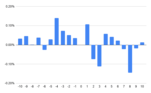
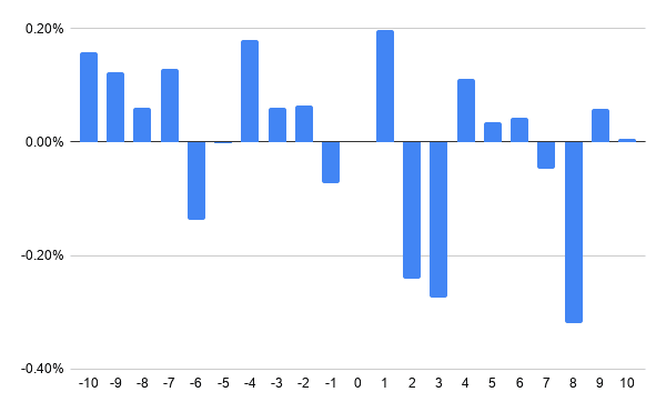
Several features are immediately visible. For both variants, day D+1 (the first trading day of the new month) produces the strongest positive average return, while days D+2 and D+3 exhibit sharp negative returns—a striking reversal that is especially pronounced for the long-short variant. Additionally, the pre-month-end window from D–10 through D–5 shows a cluster of positive average returns, consistent with the intramonth momentum cycle documented by Nathan, Suominen and Tasa (2026) at the individual-stock level. These preliminary patterns motivate the three-legged decomposition that forms the core of our empirical analysis.
5. Results
5.1 Leg One: Turn of the Month (Day D+1)
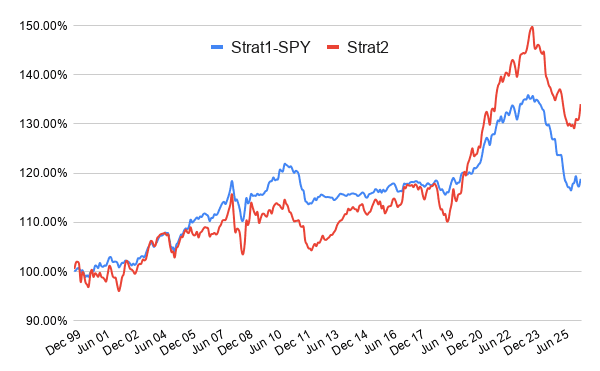
We begin with the most straightforward implementation. On the close of the last trading day of each month, we enter the momentum position (long winners, short SPY or short losers) and hold for one trading day, exiting at the close of day D+1. Figure 3 displays the cumulative equity curves for both strategy variants.
| Strategy | Perf. (p.a.) | Vol. (p.a.) | Sharpe Ratio* | Max DD | Calmar Ratio** |
|---|---|---|---|---|---|
| Strat1-SPY | 0.23% | 1.50% | 0.15 | –7.54% | 0.03 |
| Strat2 | 2.83% | 6.69% | 0.42 | –14.85% | 0.19 |
* Adjusted Sharpe Ratio assuming 0% risk-free rate.
** Defined as annualized performance divided by maximum drawdown (see Quantpedia Portfolio Analysis — Basic Overview).
The long-short variant (Strat2) captures nearly 3% annualized from a single trading day per month—a nontrivial return for a strategy that is invested under 5% of the time. The market-neutral variant is weaker, suggesting that the momentum signal is better expressed as a within-sector spread than as a sector-versus-market bet on this particular day. Both equity curves, however, exhibit meaningful drawdowns, and the Sharpe ratios, while positive, leave room for improvement. The question is whether the surrounding days can add value—or, perhaps more interestingly, whether they tell us something about the direction in which we should be trading.
5.2 Leg Two: The Post-ToM Reversal (Days D+2 and D+3)
If sector momentum “works” on day D+1, the natural next question is what happens on days D+2 and D+3. Figure 4 shows the equity curves when we hold the same momentum position (long winners, short benchmark or losers) through days D+2 and D+3 only.
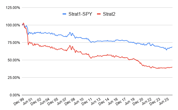
The result is unambiguously negative: both variants bleed value over the full sample, and the equity curves slope downward—precisely the mirror image of the day-D+1 pattern. This was, frankly, a surprise. Momentum signals are not supposed to reverse this quickly; the standard literature documents continuation over horizons of 3–12 months and reversal only beyond 12–18 months. A two-day reversal at the sector level is something quite different and, to our knowledge, has not been previously documented.
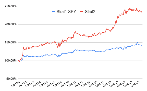
The practical implication is immediate: if holding the momentum position on days D+2 and D+3 destroys value, then reversing the position on those days should create it. Figure 5 shows the equity curves when we flip the sign—going long SPY and short the top-3 sectors (Strat1-SPY reversed) or going long the bottom-3 and short the top-3 (Strat2 reversed)—on days D+2 and D+3 only.
| Strategy | Perf. (p.a.) | Vol. (p.a.) | Sharpe Ratio* | Max DD | Calmar Ratio** |
|---|---|---|---|---|---|
| Strat1-SPY (reversed) | 0.69% | 2.25% | 0.31 | –4.86% | 0.14 |
| Strat2 (reversed) | 3.26% | 7.13% | 0.46 | –16.74% | 0.19 |
The reversed Strat2 now delivers 3.26% annualized with a 0.46 Sharpe—modestly better than the day-D+1 momentum leg itself. More importantly, the reversal confirms that the intramonth sector momentum cycle is not a monotonic phenomenon: it is a genuine oscillation, with the sign of the optimal position flipping within the first three trading days of each month. This oscillatory structure is the key empirical finding of the paper and the foundation for the composite strategy assembled in Section 5.4. It is also consistent with the flow-based framework of Nathan, Suominen and Tasa (2026): if the momentum premium is earned in the pre-month-end window through flow-driven selling of losers, month-start is precisely when that displacement unwinds.
5.3 Leg Three: Pre-Month-End Momentum (Days D–10 to D–5)
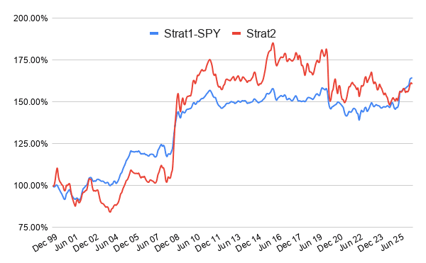
Nathan, Suominen and Tasa (2026) recently documented that individual-stock momentum strategies earn significant returns in a short window ending about four trading days before month-end, attributing the pattern to month-end cash demand—institutions “dash for cash” by selling their most dispensable positions, disproportionately losers. We test whether the same pattern appears at the sector level. Specifically, on the close of day D–10 we enter the momentum position using the trailing 252-day ranking computed at the most recent month-end—the identical ranking that drove that month’s ToM and reversal legs—and exit at the close of day D–5. Because the window reuses the existing ranking, it adds neither look-ahead nor an additional signal computation.
| Strategy | Perf. (p.a.) | Vol. (p.a.) | Sharpe Ratio* | Max DD | Calmar Ratio** |
|---|---|---|---|---|---|
| Strat1-SPY | 0.80% | 3.13% | 0.25 | –9.69% | 0.08 |
| Strat2 | 1.35% | 4.16% | 0.32 | –12.02% | 0.11 |
The effect is present at the sector level, confirming and extending the single-stock results. Returns are modest in isolation—1.35% annualized for the long-short variant—but the signal operates on a completely non-overlapping set of trading days relative to the ToM and reversal legs. This temporal independence is what makes the composite strategy viable: the three legs can be stacked without any risk of double-counting returns or compounding the same volatility exposure.
5.4 The Composite Strategy: Stitching the Cycle Together
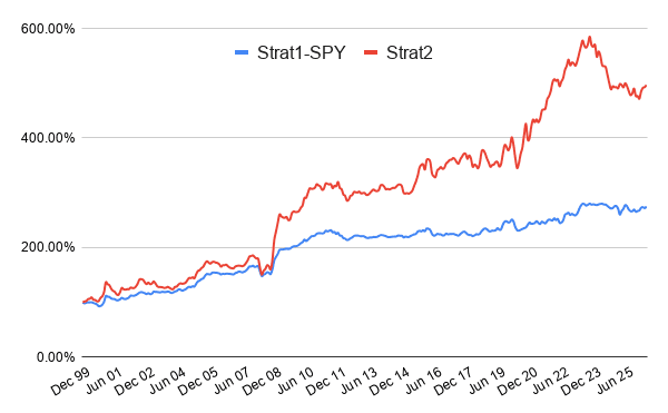
We now assemble the three legs into a single, fully specified trading calendar. Here is the monthly sequence, described in plain English:
- Days D–10 to D–5 (pre-month-end): Enter the sector momentum position—long top-3, short SPY (Strat1-SPY) or long top-3, short bottom-3 (Strat2). Exit at the close of D–5. Sit in cash for days D–4 through D–1.
- Close of the last trading day of the month: Re-rank sectors using trailing 252-day returns. Enter the new momentum position. Hold through the close of day D+1 (one trading day).
- Close of day D+1: Flip the entire portfolio. For Strat1-SPY, this means going long SPY and short the top-3 sectors; for Strat2, going long the bottom-3 and short the top-3. Hold through the close of day D+3 (two trading days).
- Close of day D+3: Close all positions. Remain in cash until the next D–10 signal.
The strategy is invested for approximately 8–9 trading days per month (roughly 40% of the time) and requires portfolio turnover only at three well-defined points: D–10, D–5/D+1 (combined rebalance), and D+3.
| Strategy | Perf. (p.a.) | Vol. (p.a.) | Sharpe Ratio* | Max DD | Calmar Ratio** |
|---|---|---|---|---|---|
| Strat1-SPY (composite) | 3.77% | 6.99% | 0.54 | –14.73% | 0.26 |
| Strat2 (composite) | 5.99% | 10.87% | 0.55 | –21.72% | 0.28 |
The composite long-short strategy (Strat2) delivers nearly 6% annualized with a 0.55 Sharpe ratio—all from a self-financing, zero-net-exposure portfolio of highly liquid ETFs that is in the market fewer than half the trading days each month. The market-neutral variant (Strat1-SPY) achieves 3.77% at a 0.54 Sharpe with a smaller maximum drawdown (–14.73%). Both variants approximately double the risk-adjusted performance of any individual leg, confirming that the three components of the intramonth cycle are genuinely complementary sources of return.
6. Discussion and Conclusions
What drives the intramonth momentum cycle? The most parsimonious explanation combines two well-established institutional mechanisms. First, turn-of-the-month cash flows—pension contributions, 401(k) deposits, fund subscriptions—create concentrated buying pressure on day D+1 that disproportionately benefits recent sector winners (which sit at the top of momentum screens and attract allocator attention). Second, the resulting overreaction is corrected on days D+2 and D+3 as liquidity providers unwind the excess demand and arbitrageurs lean against the short-term displacement. The pre-month-end leg (D–10 to D–5) reflects the same cash-demand logic running in advance of the month boundary: institutions reposition ahead of month-end, selling their most dispensable holdings—a mechanism first documented by Nathan, Suominen and Tasa (2026) for individual stocks and shown here to operate at the sector level as well. Notably, all three legs are consistent with flow-driven return variation rather than information-driven price discovery, which is precisely why the effects persist: they are a cost of doing business for large asset owners, not a mispricing that can be easily arbitraged away.
Is this just data mining? The concern is legitimate whenever a study reports multiple legs of a strategy built from the same dataset. We offer three responses. First, the three calendar windows we exploit correspond to three economically distinct mechanisms—month-end anticipation, month-start cash flows, and post-flow reversal—rather than arbitrary slicing of the calendar. Second, each leg is motivated by prior academic work (Ariel, 1987; Lakonishok and Smidt, 1988; Moskowitz and Grinblatt, 1999; Nathan, Suominen and Tasa, 2026) rather than discovered through data exploration. Third, the effect sizes are modest—the composite Sharpe ratio is 0.55, well within the range that survives realistic transaction costs for liquid ETFs—and we make no attempt to optimize holding windows or portfolio weights within the sample.
What should practitioners take away? The core message is simple: the calendar position of a sector momentum trade matters as much as the signal itself. Holding the same portfolio for an entire month dilutes the effect with noise—and reversal—from days where momentum has no edge, or worse, has a negative edge. A portfolio manager who already runs a sector momentum book can improve risk-adjusted performance materially by concentrating exposure on the days that matter and, crucially, by flipping the book for two days after each month-turn.
Takeaways
This study makes two contributions to the quantitative investment literature. First, we document a three-phase intramonth momentum cycle at the sector ETF level—momentum on D+1, reversal on D+2–D+3, and renewed momentum on D–10 to D–5—that has not previously been described as a unified phenomenon. Each phase is economically motivated by institutional flow dynamics, independently supported by prior research, and individually profitable on a risk-adjusted basis. Second, we show that compositing the three phases into a single strategy roughly doubles the Sharpe ratio relative to any individual leg, producing a 5.99% annualized return (0.55 Sharpe) in the long-short variant using exclusively liquid U.S. sector ETFs. The strategy is simple to implement, transparent in its construction, and invested fewer than half the trading days each month—an appealing combination for practitioners seeking diversifying, capacity-rich sources of return that sit outside the crowded terrain of traditional cross-sectional momentum.
Our analysis is conducted entirely at the sector level, extending findings that were previously available only for individual equities. Whether the same intramonth cycle appears in international sector indices, commodity sectors, or factor portfolios beyond momentum remains an open question—and an attractive avenue for future research.
Author: Cyril Dujava, Senior Quant Analyst, Quantpedia
Are you looking for more strategies to read about? Sign up for our newsletter or visit our Blog or Screener.
Do you want to learn more about Quantpedia Premium service? Check how Quantpedia works, our mission and Premium pricing offer.
Do you want to learn more about Quantpedia Pro service? Check its description, watch videos, review reporting capabilities and visit our pricing offer.
Do you want algorithmic access to the full Quantpedia database via the API? Subscribe to Quantpedia Pro, ask for an API key, and explore the in/out-of-sample statistics, source academic papers, and code snippets — ideal for quantitative research, systematic trading workflows, and AI model training.
Are you looking for historical data or backtesting platforms? Check our list of Algo Trading Discounts.
Or follow us on:
Facebook Group, Facebook Page, Telegram, Twitter, Linkedin, Medium or Youtube
References
Ariel, R. A. (1987). A Monthly Effect in Stock Returns. Journal of Financial Economics, 18(1), 161–174.
Lakonishok, J., & Smidt, S. (1988). Are Seasonal Anomalies Real? A Ninety-Year Perspective. Review of Financial Studies, 1(4), 403–425.
Moskowitz, T. J., & Grinblatt, M. (1999). Do Industries Explain Momentum? Journal of Finance, 54(4), 1249–1290.
Nathan, D., Suominen, M., & Tasa, J. (2026). The Intramonth Momentum Cycle. SSRN Working Paper No. 6426026. Available at: https://ssrn.com/abstract=6426026
Share onLinkedInTwitterFacebookRefer to a friend