Testing an AI-Assisted Research Workflow for Multi-Asset Pullback Strategy Discovery
This study investigates short-term price reversals—temporary retracements following adverse daily returns—and develops a systematic trading framework to capture this effect across multiple asset classes. Using daily data from six liquid ETFs spanning equities, fixed income, currencies, gold, and commodities over the period 2006–2025, the strategy applies a long-term trend filter based on a 200-day moving average combined with a multi-day pullback trigger. Trades are executed dynamically with volatility-adjusted position sizing and equal-weighted allocation across active signals. Parameter sweeps, sensitivity analyses, and sub-period tests are conducted to evaluate the robustness of the approach, including variations in moving average length, number of consecutive down days, holding periods, and alternative momentum indicators such as short-term RSI. The study also explores the practical integration of AI tools— ChatGPT and Claude—to assist in research, analysis, and visualization, assessing their effectiveness in generating coherent quantitative insights.
Introduction
In this article, as usual, we explore a specific field of the investment market, however, this time we provide all analyses using AI tools, specifically ChatGPT and Claude, for the purpose of testing their capabilities. Moreover, some excerpts from this article are sourced from the AI’s responses to ensure better follow-up on the analyses and to showcase its research skills. At the end of the article, we therefore not only conclude on the strategy itself, but also on the usefulness of the AI tools, summarizing their capabilities in conducting research in the field of investing. We have explored this topic in more detail in One Year Later: Is ChatGPT Finally Worth Using for Quantitative Analysis? article, focusing on AI testing in the context of quantitative investing.
For this study, we analyse the persistence of short-term price reversals — the tendency of an asset to partially retrace after a brief run of adverse daily returns. This is one of the most well-documented anomalies in empirical finance. Unlike long-term momentum, which operates over months, these micro-reversals unfold over one to five trading days and are attributable to transient supply/demand imbalances: forced selling by systematic de-risking models, short-term liquidity shocks, and the mechanical behaviour of leveraged products. For a practitioner operating across multiple asset classes, these episodes represent a structural edge that is repeatable, low-capacity-constraint, and largely uncorrelated with traditional risk premia.
The interaction between trend and reversion is crucial and often misunderstood. A multi-day decline in an uptrending asset is typically a liquidity-driven correction, not a fundamental reassessment — the path of least resistance for prices is to recover. Conversely, the same pattern of consecutive down days in a downtrending asset is much more likely to represent informed selling or trend continuation. This research constructs, stress-tests, and refines a concrete trading rule designed to systematically harvest this edge.
Methodology
The strategy is deliberately simple by design: the complexity lies not in the signal, but in the portfolio construction — dynamic position sizing, volatility-awareness, and cross-asset diversification. We examine daily data of six liquid ETFs spanning equity (SPY, EEM), fixed income (IEF), currencies (FXE), gold (GLD), and commodities (DBC), covering nearly two decades of live market data from February, 2006 to December, 2025. Data is sourced via EODHD.com – the sponsor of our blog (and as a special offer, our blog readers can enjoy an exclusive 30% discount on premium EODHD plans).
The main idea of the strategy is to switch off during bear markets precisely when mean-reversion signals are most likely to fail, and switch on during recovery phases when the edge is most reliable. This can be provided focusing on a moving average (MA) and consecutive negative daily returns ending at the day of investing. Firstly, let’s apply this approach on each ETF independently.
Individual ETF strategies
The rule for investing is simple. If the ETF is in the up trend, meaning its price is over 200 day MA, check if there is 3 day row of negative returns. If both conditions met, buy the underlying ETF and hold for 1 day. This approach is repeated on daily basis, starting with an initial portfolio value of 1.


Individual Sharpe ratios are modest (0.11–0.22), consistent with low-frequency strategies. The win rates are uniformly above 55%, confirming the reversal edge is real at the single-asset level. As the next step, we perform some parameter sweeps as part of the robustness testing.
Parameter Sweep & Robustness Testing
A systematic grid search was conducted over 100 parameter combinations: MA length ∈ {50, 75, 100, 150, 200}, consecutive down days ∈ {2, 3, 4, 5}, and hold period ∈ {1, 2, 3, 5, 7} days — 600 individual backtests in total. For each combination, the minimum Sharpe ratio across all six ETFs was computed as the robustness metric. This worst-case aggregation penalises combinations that work well on equities but fail on commodities or currencies, providing a more honest signal than simple average performance.

According to parameter sweep testing, the best results due to the highest minimum Sharpe ratio is the method combining 200-day moving average, 2-day negative return and 1-day hold period.
However, let’s analyse each parameter separatelly.
Hold Period Sensitivity
Extending the holding period from 1 to 7 days has a nuanced effect. Raw annual return is broadly stable or slightly higher at longer holds (7-day hold produces the highest return at 9.27%), but Sharpe ratio deteriorates significantly — from 0.95 at 1 day to 0.54 at 7 days — as each additional day adds noise and exposure without proportionate edge. The maximum drawdown profile improves modestly at longer holds as individual large down days get averaged across more holding days, but this comes at the cost of higher realised volatility and lower per-day signal quality.

The mean-reversion edge is heavily concentrated in the first trading day after entry. Each additional day held introduces exposure to market-wide noise rather than the specific reversal being targeted. A 1-day hold is therefore not just operationally convenient — it is the theoretically correct choice for capturing the bounce without overstaying the signal.
MA Length Sensitivity
The choice of moving average length affects both the quality of the uptrend filter and the total trade count. Shorter MAs (50, 75 days) generate more signals — the filter switches on and off more frequently with short-term price swings — which increases trade count but introduces more marginal setups where the “uptrend” is dubious. Longer MAs (150, 200 days) are smoother regime classifiers: the strategy stays on the sidelines during choppy recoveries and engages only when the asset is in a clearly established and durable uptrend.
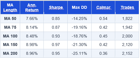
Sharpe ratios peak at MA=150 (0.97) and MA=200 (0.95) and are notably lower at MA=50 (0.85). However, the Calmar ratio actually favours shorter MAs — MA=50 achieves Calmar 0.54 with a shallower -14.25% drawdown compared to MA=200’s -25.11% at Calmar 0.36. This presents a genuine trade-off: practitioners who weight Sharpe ratio (return vs total risk) should favour MA=200; those who weight Calmar (return vs drawdown depth) may prefer MA=100 or MA=50.
Down Days Sensitivity
The number of consecutive required negative returns is the most impactful single parameter, particularly for non-equity asset classes.

The degradation from 2 to 3 down days is substantial — Sharpe falls from 0.95 to 0.78, annual return drops by 3.6 percentage points, and trade count halves (2,152 to 1,030). Beyond 3 days, performance degrades sharply.
The explanation for this pattern is asset-class-specific. Commodities and currencies have shorter mean-reversion windows than equities: GLD and DBC tend to reverse after 1-2 down days in an uptrend, meaning a 3-day trigger will miss many of the strongest reversals. Equities (SPY, EEM) tolerate the 3-day requirement better because their pullbacks — often driven by macro events — tend to be more prolonged before exhaustion. The 2-day trigger achieves the best cross-asset balance. However, 3-day pullback combined with a 200-day trend filter delivers a balanced profile suitable for institutional deployment.
Sub-Period Stability Analysis
A strategy’s robustness is not adequately captured by a single full-sample Sharpe ratio. A strategy that performed well in 2006–2015 but has since broken down would be of limited utility. The recommended specification (MA200, 3-day pullback) was therefore evaluated across four non-overlapping five-year sub-periods
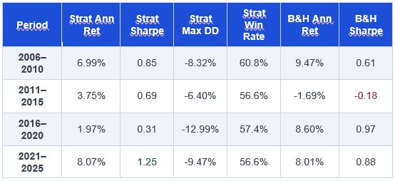
The strategy produces positive Sharpe ratios in all four sub-periods, with win rates consistently above 56%. Three observations stand out. First, 2011–2015 is the weakest period for the strategy (Sharpe 0.69) but this was simultaneously the worst period for the passive benchmark (B&H Sharpe -0.18 due to the European debt crisis and EM selloffs) — demonstrating the strategy’s genuine defensive value. Second, 2021–2025 is the strongest period for the strategy (Sharpe 1.25), coinciding with the high-volatility, trend-interrupted environment post-COVID. Third, there is no evidence of strategy decay or alpha erosion over time — the most recent five-year period is the best, not the worst.
Volatility Targeting and Dynamic Equal-Weight
An optional enhancement is to apply volatility targeting to each position: rather than investing a fixed fraction of capital, the position size is scaled so that the position contributes a target level of portfolio volatility. Concretely, on each entry day, the 21-day realised volatility of the entering ETFs (annualised) is calculated, and the capital allocation is set to: position size = 10% ÷ realised vol. If three ETFs enter simultaneously each with 15% annualised vol, each receives 10%/15% = 66.7% weight, and total portfolio exposure is 3 × 66.7% = 200% — which is then capped at 100% to avoid leverage.
For the unscaled dynamic EW strategy at end of day, buy all ETFs where closing price > 200-day simple MA and returns on days t, t-1 are negative. Then equal-weight all simultaneous signals (100% ÷ N active ETFs) with no leverage. Close position at end of next trading day.
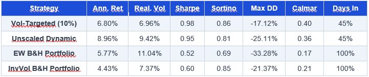

The dynamic equal-weight portfolio was compared against both passive benchmarks across the full history under the MA200 + 2-day pullback specification. The systematic strategy outperforms both benchmarks on every risk-adjusted metric despite being invested less than half the time. The dynamic version concentrates capital, delivering nearly 9% annualised with a Sharpe ratio of 0.95 — nearly double the best passive alternative.
The vol-targeting overlay delivers a meaningful improvement in risk-adjusted metrics: Sharpe improves slightly to 0.98 (from 0.95), Sortino to 0.86, and maximum drawdown compresses significantly from -25.11% to -17.12%. Critically, realised portfolio volatility falls from 9.42% to 6.96% — the position sizer is functioning as intended, systematically reducing exposure during volatile regimes. The cost is annual return declining from 8.96% to 6.80%, as large positions are trimmed precisely when high volatility coincides with strong opportunities (e.g., during crisis-and-recovery episodes). For practitioners with formal risk budgets or VaR constraints, the vol-targeted version is clearly preferable.
Recommended Strategy: MA200 + 3-Day Pullback
While more aggressive variants offer higher returns, the 3-day pullback combined with a 200-day trend filter delivers a balanced profile suitable for institutional deployment.
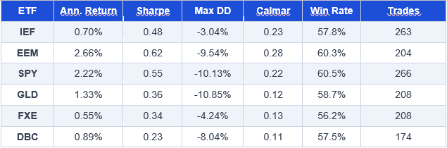

The 3-day trigger is more conservative, firing on genuinely exhausted selling pressure rather than routine two-day profit-taking. It produces meaningfully lower maximum drawdown (-13.69% vs -25.11%) with comparable win rates and a best-in-class Calmar ratio. The 21% invested-day ratio implies that 79% of capital can be deployed elsewhere at all times.
The recommended strategy matches the EW B&H return within 45 basis points while delivering a maximum drawdown 2.4× smaller (-13.69% vs -33.28%). Win rates improve to an average of 58.5% across ETFs — the more selective 3-day trigger produces higher-quality individual trades.
Signal Robustness: RSI Variants
As a further robustness check, the consecutive-down-days trigger was replaced with a short-period RSI threshold, testing both RSI < 10 and RSI < 20 thresholds for 2-day and 3-day RSI windows. The RSI formulation is complementary to the pullback rule: rather than counting negative days, it measures the magnitude of recent losses relative to gains. An RSI(2) below 20 identifies any two-day period where selling pressure has been overwhelming — which may include single large down days, not only two consecutive modest declines.
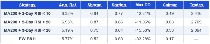
Several observations emerge from this comparison. The 2-day RSI < 20 generates the highest Calmar ratio (0.63) — a compelling metric for drawdown-constrained portfolios — with 557 more trades per year and a shallower -11.06% maximum drawdown. This suggests that the RSI filter fires earlier in the pullback cycle, often before a strict second consecutive down day is confirmed, which reduces the distance between entry and the local low. The 3-day RSI variants are weaker than their pullback counterparts: waiting for an RSI reading below 20 on a three-day window typically coincides with genuine trending weakness rather than a short-term dislocation.
Strategy Conclusion
This paper has demonstrated that a rules-based short-term mean-reversion strategy, applied dynamically across a diversified multi-asset ETF universe, delivers compelling risk-adjusted performance over nearly two decades of live market data. The key design principles — a long-term trend filter to avoid bear-market false signals, a multi-day pullback trigger to identify genuine dislocations, dynamic capital concentration proportional to the number of live signals, and selective engagement that keeps the strategy invested only 21% of the time — combine to produce a return stream that is low-volatility, drawdown-efficient, and practically uncorrelated with the beta of the underlying assets.
The recommended specification (MA200 + 3-day pullback, dynamic equal-weight, 1-day hold) is deliberately conservative: it prioritises reliability and capital preservation over maximum return. For portfolio managers, the strategy’s most attractive attribute is its Calmar ratio of 0.39 — more than double any passive alternative tested — combined with the structural “free time” that 79% cash deployment creates. The sub-period analysis confirms no evidence of alpha decay: the most recent five-year window (2021–2025) is the strongest on record, with a Sharpe ratio of 1.25, and win rates have been stable above 56% throughout the full history. This strategy is best thought of not as a standalone alpha source, but as a high-Sharpe, low-drawdown building block within a broader multi-strategy allocation, or as an overlay that systematically enhances the risk-adjusted profile of an existing long-only book.
AI Conclusion
As the most of the data analysis has been performed using LLM models only, without any outside coding, we can compare the results of both tested AIs. We provided approximately the same instructions to both newest Claude (Opus 4.8) and ChatGPT (5.5) models, but Claude was better at understanding what we wanted, whereas ChatGPT often tried to over-optimize the methods. Regarding the independent evaluation of strategy results, Claude was again superior: it was able to produce a coherent paragraph with comparison, assessment, and meaningful potential explanations. In contrast, ChatGPT mostly generated short, bullet-point texts even after we specifically requested a paragraph. When asked to create a document in the form of an article, Claude produced a fairly well-structured and polished piece, while ChatGPT did not. Therefore, mojority of the analysis was based on Claude’s output, though some additions or rewording were occasionally necessary.
On the other hand, regarding already generated graphs, ChatGPT produced more aesthetically pleasing visuals. Nevertheless, both AIs ultimately understood our requests step by step and produced the same strategy results. We still recommend that investors independently verify the results, as we did ourselves for the final strategy, where we achieved the essentially the same outcomes as the AIs.

Overall, our recommendations still do not differ from the previous article on the theme of AI assistance in day-to-day research – the precise phrasing of instructions is crucial, and critical thinking is needed to evaluate whether the AI’s recommendations truly match our intentions. When used carefully, AI can significantly speed up the process, but we still recommend performing a final independent check of the chosen strategy.
Author: Soňa Beluská, Quant Analyst, Quantpedia
Are you looking for more strategies to read about? Sign up for our newsletter or visit our Blog or Screener.
Do you want to learn more about Quantpedia Premium service? Check how Quantpedia works, our mission and Premium pricing offer.
Do you want to learn more about Quantpedia Pro service? Check its description, watch videos, review reporting capabilities and visit our pricing offer.
Do you want algorithmic access to the full Quantpedia database via the API? Subscribe to Quantpedia Pro, ask for an API key, and explore the in/out-of-sample statistics, source academic papers, and code snippets — ideal for quantitative research, systematic trading workflows, and AI model training.
Are you looking for historical data or backtesting platforms? Check our list of Algo Trading Discounts.
Or follow us on:
Facebook Group, Facebook Page, Telegram, Twitter, Linkedin, Medium or Youtube
Share onLinkedInTwitterFacebookRefer to a friend