Delta hedging is a trading strategy that aims to reduce the directional risk of short option strategy and reach a so-called delta-neutral position. It does so by buying or selling small increments of the underlying asset. Similarly, grid trading is a trading strategy that buys/sells an asset depending on its price moves. When the price falls, it buys and sells when the price rises a certain amount above the buying price. This article examines the similarities between delta hedging and grid trading. Additionally, it analyzes numerous versions of grid trading strategies and compares their advantages and disadvantages.
Introduction to delta hedging
Option’s delta tells us how much the value of an option rises/ falls with the move in the stock’s price. For example, if the stock call option has a delta of 0.3 and the underlying stock increases by $1 per share, the option value will rise by $0.3 per share. If an investor wants to reduce the risk linked to the price changes, he can take a position in the option together with the underlying asset, with the weight corresponding to the delta of said option. However, this only reduces the risk at one moment. Therefore, to minimize the risk in the extended period, the investor should continuously buy/sell a percentage of the underlying asset corresponding to the option’s price movements and its delta – the investor must perform delta hedging.
Advanced options strategies trade volatility via delta-neutral strategies. A delta-neutral position is one in which the overall delta is zero. This approach minimizes the options’ price movements in relation to the underlying asset. An example is a short straddle position.
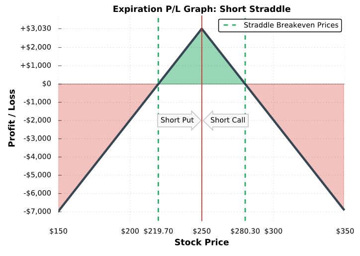
An investor holding a short straddle position has at the beginning a delta of 0 and is losing when the option’s underlying price moves significantly in any direction. The investor is essentially short volatility. How will delta-hedging work in this example? When the price of the underlying increases, the investor must neutralize the delta of the overall option strategy and buy a small fragment of the underlying. On the other hand, when the price of underlying decreases, the investor must sell some underlying.
If investors were to continuously buy/sell the underlying asset without any transaction costs, they would have a perfect hedge. However, it is impossible to trade continuously or without transaction cost in reality. So, the rebalancing is done on a periodic basis (it can be done multiple times per day, but usually once a day or once a week), and thus the investor is constantly exposed to risk.
Essentially, delta hedging of a short straddle option position is a strategy that continuously buys when the price of the underlying goes up and sells when the price goes down. It’s a long volatility strategy, similar to time-series momentum or trend-following strategies. Usually, average trade incurs a small loss (as we are buying at a little higher price than selling). But usually, the overall loss from the delta hedging is smaller than the premium we receive from sold options, and hedging increases the Sharpe ratio of short volatility strategies as it protects against large directional moves.
Grid Trading
Grid trading is an investment strategy that buys an asset when its price falls and sells when it rises a certain amount above the buying price. Therefore, this strategy is basically reverse to delta hedging.
If an option trader sold a put option, they could apply a delta hedge. So, if the underlying asset’s price is falling, the investor sells a percentage of the underlying asset. On the other hand, if an investor doesn’t sell option and just applies a grid trading strategy, they stand on the opposite side of delta hedger’s trades – they are buying an asset when the price is falling.
To put it simply, an investor holding a short straddle position is short volatility. An investor who applies delta hedging trades (without short option position) is long volatility (profits when price continues to move in one direction). And lastly, an investor who applies grid trading is in a similar position to the investor who holds the short straddle position but without the need to use the options – he has a short volatility position, he profits if prices do not move strongly in one direction.
Grid trading – analysis
Let us now continue and discuss various forms of daily rebalanced grid trading strategies. We focus on numerous approaches and analyze the pros and cons of each one. Finally, we describe multiple grid trading strategies and illustrate their results. As we have explained in previous paragraphs, grid trading is essentially short volatility strategy and this understanding gives us better insight into the results of different variants.
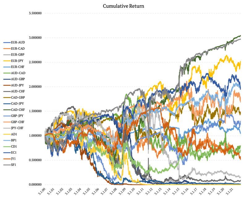
We analyze futures on six currencies, including AD1 (Australian Dollar), BP1 (British Pound), CD1 (Canadian Dollar), EC1 (Euro), JY1 (Japanese Yen), SF1 (Swiss Franc), as well as 15 cross-currency pairs between these currencies from 4. Jan 1999 till 30. Nov 2021. It is important that we use futures and not just spot exchange rates because the price of a future includes interest rates.
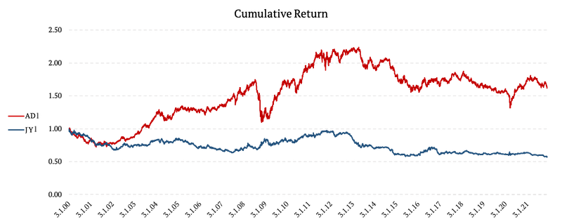
For example, currencies of countries with high-interest rates, such as Australia, tend to move significantly more than currencies of countries with low-interest rates, such as Japan. Let’s look at the following figure, which illustrates the cumulative return of each currency’s futures.
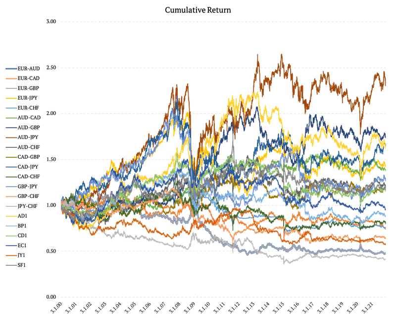
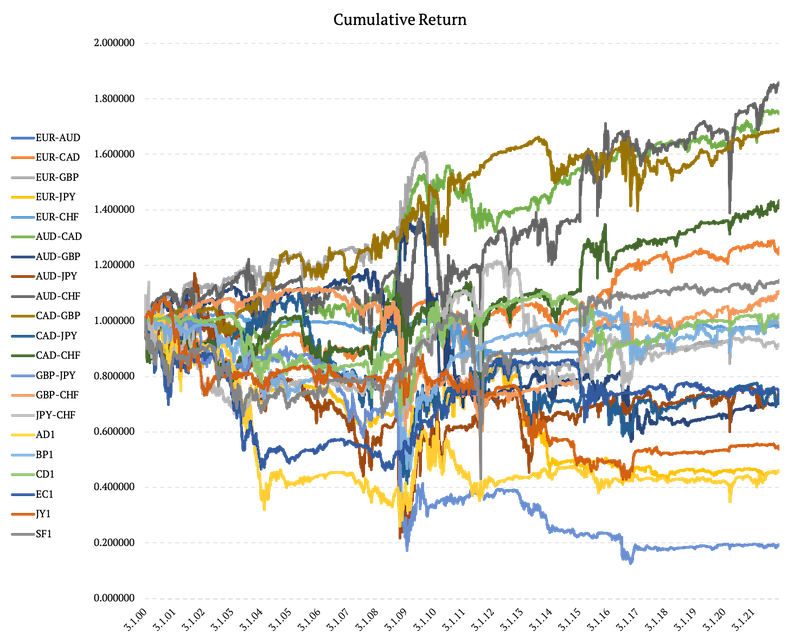
The following figure shows the equity curves of all the futures and the 15 cross-currency pairs.
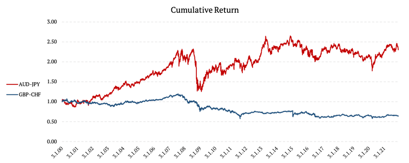
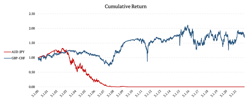
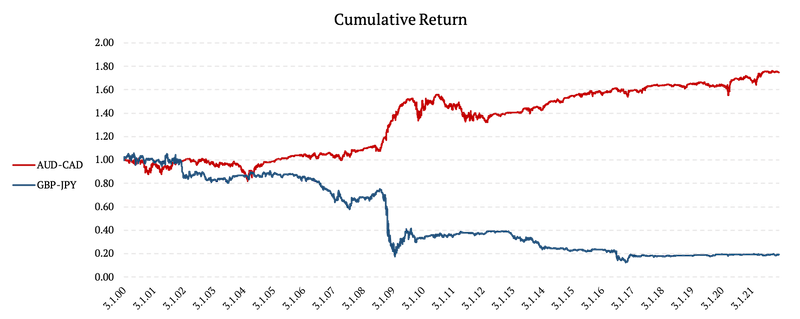
Lastly, we present a figure illustrating two of the synthetic cross-currency pairs. This figure shows how cross-currency pairs of countries with substantially different interest rates, such as Australia and Japan, tend to drift significantly more than the cross-currency pairs of countries with similar interest rates, such as Great Britain and Switzerland.
As we can see, it’s really important to pick the correct underlying currency pair to use for the grid trading strategy. But the question of which pair to pick will be answered in some other later article. In this article, we will take a look at “reference price”.
Reference Price in Grid Trading
One of the most important things is to set the so-called “reference price”. An investor decides whether to go long or short based on the set reference price. The strategy goes short if today’s price is greater than the reference price.
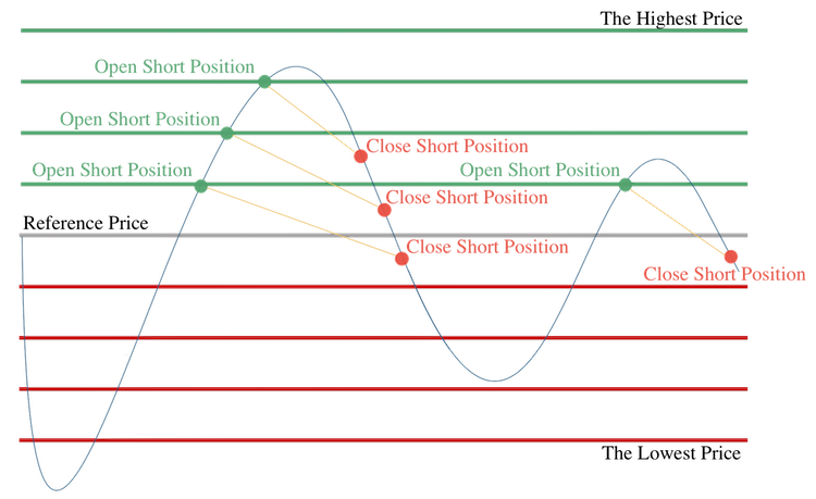
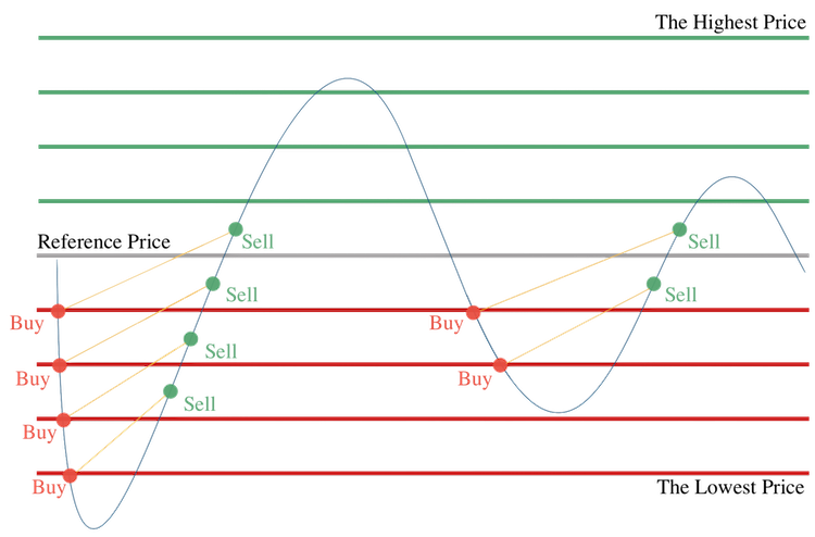
On the other hand, the strategy goes long when today’s price is lower than the reference price.
The grid trading strategy usually uses significant leverage, and it is also calculated based on the reference price. In our analysis, we use the leverage of up to 10:1, and position size is calculated as:
position size = 10 x ( 1 – today’s price / reference price )
There are many ways one can set the reference price. This article examines three of the simpler strategies so that the next one can analyze more complex approaches on how to set the reference price.
Each grid trading variant that’s described later is rebalanced daily. Each trading day, we go short underlying at the close if the close price is higher than the reference price, and we go long if the current close price is lower than the reference price. The amount invested is proportional to the difference between the current price and reference price multiplied by the leverage. Essentially, we average down into position if the price decreases and increase shorting position if the price rises.
Fixed reference price
The first strategy we introduce in this article is the simplest one. We set the reference price as the price at the beginning of the observed period. So, for each currency futures and cross-currency futures pair, it is the price on 4. Jan 1999. This approach is very time-sensitive. Meaning the result of such a strategy very strongly depends on the asset’s price on the first day.
As the price rises relative to the reference price the investor opens the short position. However, if the price falls below the reference price, the investor opens the long position.
The following figure shows the performance of grid trading strategy on synthetic cross-currency pairs of Australia – Japan, and Great Britain – Switzerland. As we can see, the performance of the Japan Yen – Australian Dollar falls dramatically after the initial two and a half years. This currency pair trends strongly and it not a very good candidate for short volatility strategy like grid trading. On the other hand, the performance of the grid trading strategy applied on Great British Pound – Swiss Franc looks relatively better.
Overall, we can say that having a fixed reference price does not convey the best results. Furthermore, this approach is very time-sensitive, and thus the performance of the whole strategy depends solely on the price set at the beginning. Lastly, the figure below shows all of the analyzed equity-curves.
The figure shows that the majority of portfolios have a very small or negative annualized return, in addition to high volatility and significant drawdowns. Only a few of the currency pairs are stable enough so that the grid trading strategies with fixed reference prices have attractive equity curves.
Moving reference price
Another approach we can take is to move the reference value in time. In this case, the grid trading strategy sets the reference price as the price from 250-days ago. This approach is not as time-sensitive as we reset the reference value every day.
The grid trading strategy for cross-currency pairs of countries with similar historical movements of levels of interest rates, such as Canada and Australia, performs well compared to the cross-currency pairs of countries with different historical movements of interest rates such as Great Britain and Japan.
But overall, we must again have a method to select promising currency pairs as most of the equity curves for grid trading strategies are not so attractive:
Monthly-reset reference price
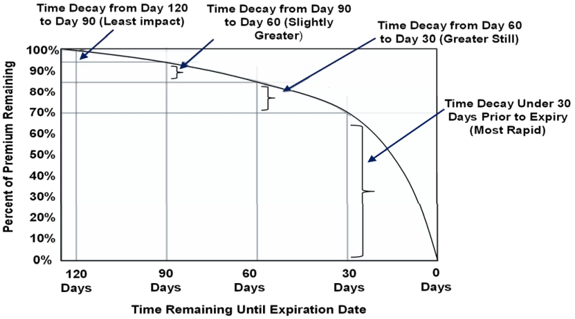
The idea behind the last analysis we present in this article is inspired by option trading. As explained in the theoretical intro, the grid trading strategy is essentially a short volatility strategy. Option writing strategies usually sell options with a shorter time to maturity as price decay is faster the closer to maturity the option is.
With similar reasoning, how do the grid trading strategies perform on individual currencies if we reset the reference price on a monthly basis?
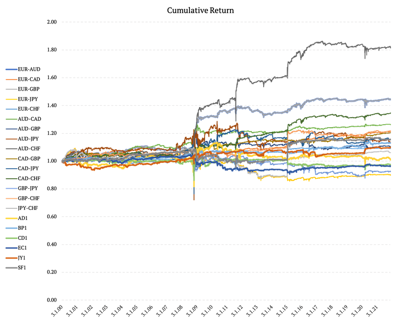
Average equity curve improved, we do not have so much equity curves in deep drawdowns and some of the pairs have interesting performance. So how does a daily rebalanced equally-weighed portfolio of all grid trading strategies on all of the currency futures and the cross-currency pairs look like?
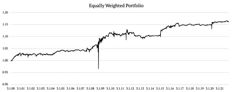
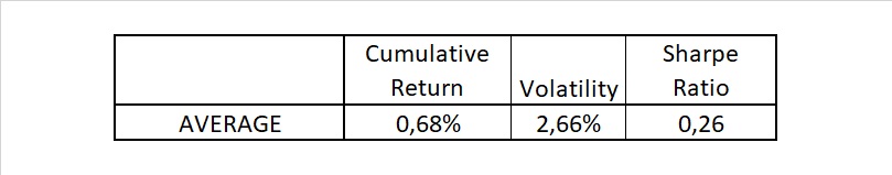
The average performance is low, but volatility is also low, and the average Sharpe Ratio is positive, and we can easily improve performance by increasing leverage. Overall, it seems that we are moving in the right direction, but there are more aspects of grid trading strategies that we can investigate than just the reference price.
Performance of grid strategies strongly differs among different currency pairs as they move between trending and sideways periods. So the next logical step is to try to distinguish between those two market states and adjust individual grid trading strategies accordingly. How? That would be the topic in one of our future articles.
Author:
Daniela Hanicova, Quant Analyst, Quantpedia
Are you looking for more strategies to read about? Sign up for our newsletter or visit our Blog or Screener.
Do you want to learn more about Quantpedia Premium service? Check how Quantpedia works, our mission and Premium pricing offer.
Do you want to learn more about Quantpedia Pro service? Check its description, watch videos, review reporting capabilities and visit our pricing offer.
Are you looking for historical data or backtesting platforms? Check our list of Algo Trading Discounts.
Or follow us on:
Facebook Group, Facebook Page, Twitter, Linkedin, Medium or Youtube
Share onLinkedInTwitterFacebookRefer to a friend