Alternative Market Signals: Investing with the Box Manufacturing Index
Investors are increasingly exploring alternative indicators to gain an edge in financial markets. Traditional signals, such as earnings reports or macroeconomic data, often come with delays or may already be priced in. As a result, unconventional metrics have attracted attention. For example, recent focus has been on construction inventory statistics, where large stockpiles have been interpreted as a signal of weakening demand for construction activity. This, in turn, may reflect broader consumer and corporate hesitancy to spend, implicitly suggesting a potential decline in asset prices. In this article, we examine a different type of alternative indicator: the Producer Price Index (PPI) for the Corrugated and Solid Fiber Box Manufacturing industry, including corrugated boxes and pallets. Our motivation is to evaluate this index’s effectiveness as a predictive signal for the S&P 500 ETF, sector-specific ETFs, and individual stocks such as Amazon (AMZN), one of the largest consumers of materials tracked by this index. We present several investment strategies that incorporate this indicator and assess whether it can enhance risk-adjusted returns.
Motivation
Relying exclusively on traditional prediction inputs such as stock prices, quarterly earnings reports or forward guidance comes with a structural limitation. Financial markets usually incorporate expectations long before the information becomes public. As a result, much of the anticipated performance is already reflected in the price by the time earnings are released. Entering positions shortly before these announcements essentially turns into a bet on whether the results will outperform what is already priced in. This introduces a level of event-driven risk that is difficult to manage and offers little foundation for building systematic strategies with stable risk profiles.
This creates a clear incentive to explore indicators that capture real economic activity without being immediately absorbed by market expectations. With the PPI for Corrugated and Solid Fiber Box Manufacturing, we build on an intuitive idea. Rising production or consumption of packaging materials signals higher demand for these inputs. Companies purchase more corrugated boxes and pallets when they need to ship a larger volume of goods. Increased packaging demand therefore serves as a proxy for growing order flows, stronger consumer activity and higher throughput across supply chains. These conditions often accompany periods of economic expansion, which tend to support corporate revenues and earnings. If this relationship holds, an upward trend in packaging-related PPI data may precede rising prices in broad market ETFs, sector-specific ETFs or individual stocks such as Amazon.
Data overview
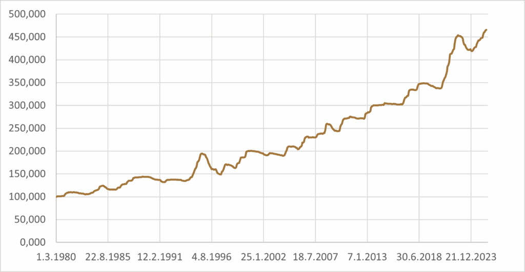
The analysis relies entirely on monthly data. This frequency is dictated by the characteristics of our primary indicator, the PPI for Corrugated and Solid Fiber Box Manufacturing, which is released only once per month and often not on a fixed schedule. As a result, all strategy decisions are implemented with a one-month delay and evaluated at monthly intervals.
Our predictor series is available from March 1980, providing a long historical window for testing. For comparison with market instruments, we include several widely used exchange-traded funds and individual equities, each with its own start date based on data availability. Amazon (AMZN) enters the analysis from February 2000. Sector ETFs are incorporated beginning in December 1998, specifically Consumer Discretionary (XLY), Utilities (XLU), Health Care (XLV) and Consumer Staples (XLP). These funds represent distinct segments of the economy and offer a structured way to observe how different sectors respond to changes in underlying economic activity. The broad market proxy SPY, tracking the S&P 500, is included from December 2004. For a low-risk asset for times of uncertainty, we use BIL, a short-term Treasury ETF, available from June 2007, which serves as a cash-like alternative within our strategy tests.
Several additional ETFs were reviewed during the exploratory phase, including Industrials (XLI), Retail (XRT) and the Online Retail ETF (ONLN). Their results did not differ meaningfully from the sectors already presented, and in some cases the available history was too short to provide robust conclusions. For clarity and relevance, they are therefore not included in the final set of instruments discussed in this article.
Data were pulled from EODHD.com – the sponsor of our blog. EODHD offers seamless access to +30 years of historical prices and fundamental data for stocks, ETFs, forex, and cryptocurrencies across 60+ exchanges, available via API or no-code add-ons for Excel and Google Sheets. As a special offer, our blog readers can enjoy an exclusive 30% discount on premium EODHD plans.
AR models and their limitations
One natural idea was to explore autoregressive models, since it is not the level of the indicator that appears most relevant, but its change. This naturally leads to working with first differences. If month-to-month movements capture meaningful shifts in economic activity, one could construct a rule in which deviations of a certain size generate buy or sell signals. Conceptually, this resembles creating a band around the differenced series and reacting whenever the index moves outside that band.
Although appealing, this approach carries an important implicit assumption. It works only if the variability of the series remains roughly constant over time. In statistical terms, the method assumes homoskedasticity. In our case, however, the variability of the PPI differences does not remain stable. Over the long sample, the fluctuations become larger and the amplitude of movements increases. When the variance grows, the differenced series begins to produce a significant amount of noise, making the signals unstable and reducing the reliability of any band-based strategy. Instead of capturing meaningful changes in economic activity, the model increasingly reacts to the changing scale of the data itself.
Incorporating this time-varying volatility into a predictive model significantly complicates its design. The presence of heteroskedasticity means that fixed-threshold rules or static bands no longer translate consistently across the entire sample, and the model must account for the changing scale of fluctuations. Even attempts to explicitly introduce time-dependent variance adjustments do not necessarily improve predictive power, because the signal-to-noise ratio may still remain low and the underlying economic relationships may not be captured simply by scaling the series. As a result, strategies based on naive autoregressive frameworks or static thresholds can lose reliability when applied to data with evolving variability.
MA models
Following the negative experience with autoregressive models, attention turned to moving average (MA) approaches. Unlike AR models, MA models are less sensitive to heteroskedasticity because they smooth the series locally, making the long-term structure of the variance function largely irrelevant. Two natural directions emerge when working with MA models. The first is to track N-month maxima, while the second is to compare values against the N-month moving average.
Strategies based on both approaches were tested, but N-month maxima performed relatively poorly. This appears to be because maxima primarily capture trends rather than short-term deviations, which are the focus of our predictive efforts. By the time a local maximum is reached, the opportunity for early signal detection is already partially lost. In contrast, comparing the current value to the N-month moving average allows us to identify significant deviations from the trend, effectively capturing unusual movements relative to the expected level. From a broader perspective, this makes sense, as smoothing the series provides a clearer view of the underlying dynamics. Based on these considerations, we adopt the moving-average-based approach as the foundation for the strategies presented in this article.
Switch models and economic uncertainty
In several of our previous articles (for example, about BTC ETFs or VIX-based assets), we have employed what are commonly referred to as switch strategies. These strategies are based on the principle of dynamically adjusting portfolio allocations according to the signals generated by one or more indicators. Rather than maintaining a fixed allocation across all assets or sectors, the strategy “switches” between different portfolios depending on the observed state of the indicator.
SPY models as a naive benchark
Armed with these insights, we can now turn to empirical analysis. To start, we construct a set of relatively simple benchmark tests to evaluate the performance of our approach. As an initial exercise, we apply the strategy to the SPY ETF, which tracks the S&P 500 and serves as a broad-market reference. By testing on SPY first, we establish a baseline understanding of how the indicator-driven switch strategy behaves in practice, before extending the analysis to sector-specific ETFs or individual stocks. This initial benchmark helps highlight both the potential benefits and the limitations of our method in a straightforward, controlled setting.
2. Close position in SPY, when box predictor reaches its moving average.
3. If no position is opened, stay in cash.
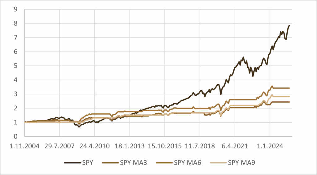
Table 1: Performance metrics of SPY-based switch strategies.
| PORTFOLIO | CAR p.a. | VOL p.a. | MAX DD | SHARPE | CALMAR |
|---|---|---|---|---|---|
| SPY portfolio | 10.48% | 14.84% | -50.76% | 0.71 | 0.21 |
| 3M SPY portfolio | 4.41% | 10.68% | -27.62% | 0.41 | 0.16 |
| 6M SPY portfolio | 6.14% | 9.94% | -19.44% | 0.62 | 0.32 |
| 9M SPY portfolio | 5.16% | 8.25% | -19.44% | 0.63 | 0.27 |
The results clearly show that applying this strategy directly to SPY is not a promising approach (in terms of return). The reason lies in the structure of the S&P 500 itself. As a broad market index, it contains companies from virtually every sector, many of which are only marginally affected by fluctuations in consumer-sensitive industries. Although some portion of the index naturally reflects changes in consumer demand, the effect is diluted across a wide and heterogeneous set of constituents. As a result, the signal derived from packaging-related PPI data does not translate into sufficiently strong or timely movements in the index. In addition, the strategy remains inactive for extended periods, avoiding certain market downturns but at the same time failing to capture enough of the index’s growth phases. This combination of weak linkage to the underlying indicator and insufficient participation in rising markets leads to overall performance that is far from compelling when applied to SPY.
Even though the overall performance on SPY was not particularly strong, the results reveal an important pattern. The strategies improved risk-adjusted metrics and therefore are a possible starting point for our analysis.
Switch models for sector ETFs
Earlier results showed that introducing a switch model can improve risk-adjusted performance, but the approach used so far had two notable limitations. First, the defensive side of the switch rule remained unchanged throughout the analysis, which restricted the model’s ability to do at least something in different market environments. Second, by applying the strategy to the broad S&P 500, we diluted the economic signal that originates from consumer-dependent activity. This reduced the effectiveness of the indicator and limited the strategy’s potential.
A natural next step is therefore to shift the focus from the entire market to sector-specific ETFs. These offer more direct exposure to the economic mechanisms our indicator captures. By placing Consumer Discretionary (XLY) on the offensive side and Consumer Staples (XLP) on the defensive side, we align the strategy with the fundamental trend we aim to exploit: discretionary spending expands strongly in favorable conditions, while staples provide resilience during downturns. It is also reasonable to test longer moving-average windows to capture more stable dynamics and potentially produce more robust results. This combination allows us to better match the indicator with the sectors most sensitive to the underlying economic activity and thereby enhance the performance of the switch model.
2. Close position in XLY, when box predictor reaches its moving average. Open position in XLP.
3. Close position in XLP, when box predictor goes above its 3M/6M/9M/12M/24M/36M MA.
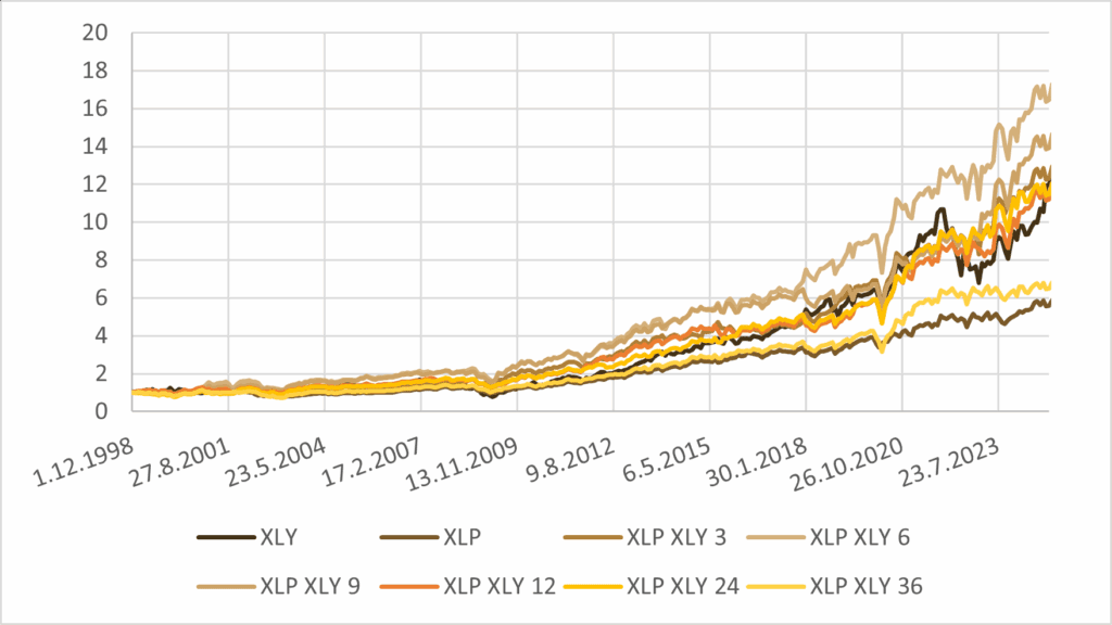
Table 2: Performance metrics of XLY – XLP switch strategies.
| PORTFOLIO | CAR p.a. | VOL p.a. | MAX DD | SHARPE | CALMAR |
|---|---|---|---|---|---|
| XLY portfolio | 9.70% | 19.24% | -54.93% | 0.5 | 0.18 |
| XLP portfolio | 6.73% | 12.23% | -32.82% | 0.55 | 0.21 |
| 3M XLY – XLP switch portfolio | 9.92% | 15.98% | -33.95% | 0.62 | 0.29 |
| 6M XLY – XLP switch portfolio | 11.12% | 16.23% | -33.02% | 0.69 | 0.34 |
| 9M XLY – XLP switch portfolio | 10.43% | 15.84% | -28.05% | 0.66 | 0.37 |
| 12M XLY – XLP switch portfolio | 9.54% | 15.05% | -30.19% | 0.63 | 0.32 |
| 24M XLY – XLP switch portfolio | 9.64% | 14.57% | -28.05% | 0.66 | 0.34 |
| 36M XLY – XLP switch portfolio | 7.33% | 13.81% | -36.06% | 0.53 | 0.20 |
The sector-level results reveal that the switch model becomes a highly effective decision tool when applied to XLY and XLP. The improvements are visible across all key metrics: overall returns rise, the Sharpe ratio increases, and the Calmar ratio strengthens as well. This suggests that aligning the model with consumer-driven economic cycles provides a much cleaner signal than operating at the broad-market level.
There is, however, one important caveat. Such a strong improvement raises the possibility that the strategy is partially overfitted to the specific sector pair or the selected parameter windows. To address this concern, it is useful to broaden the scope of the analysis and explore ensemble-type approaches—models that combine several switch strategies at once. By aggregating multiple signals, we may reduce sensitivity to any single sector, time window, or parameter choice, and potentially obtain more stable performance out-of-sample.
As a next step, we construct portfolios that evenly combine multiple moving-average windows to reduce sensitivity to any single parameter choice. Specifically, we create one set of portfolios that averages signals across 3- to 12-month windows, and another set that spans 3- to 36-month windows.
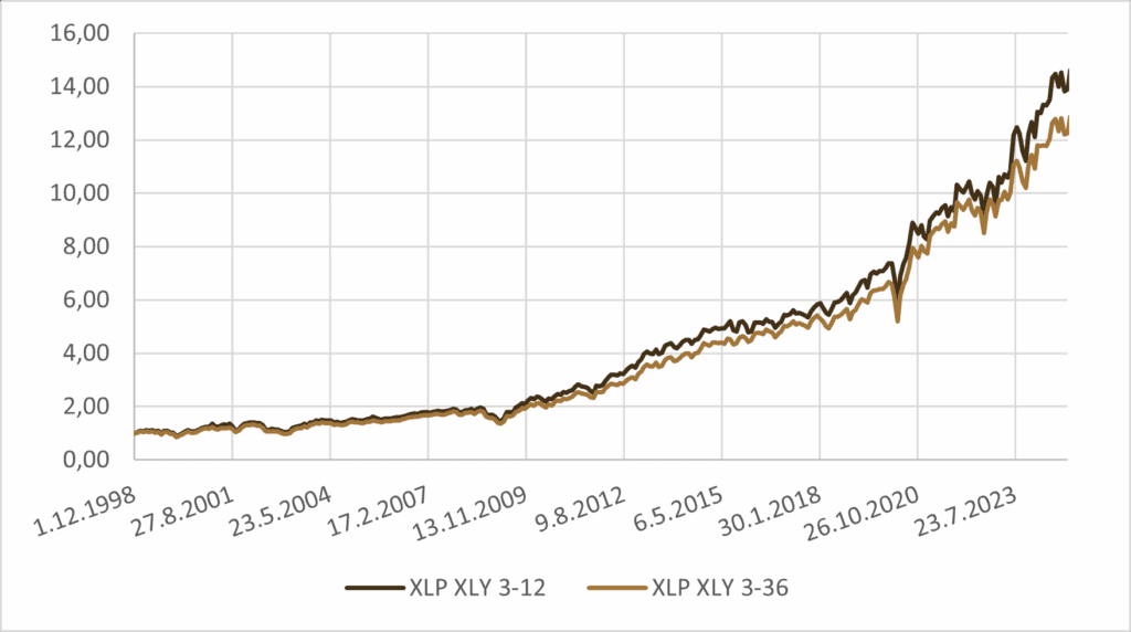
Table 3: Performance metrics of combining XLY – XLP switch strategies.
| PORTFOLIO | CAR p.a. | VOL p.a. | MAX DD | SHARPE | CALMAR |
|---|---|---|---|---|---|
| 3+6+9+12M XLY – XLP switch portfolio | 10.42% | 14.76% | -26.57% | 0.71 | 0.39 |
| 3+6+9+12+24+36M XLY – XLP switch portfolio | 9.90% | 13.68% | -27.16% | 0.72 | 0.36 |
Combining these multiple moving-average strategies reduces both risk and drawdowns, making the approach particularly effective. By diversifying across different time windows, the portfolio becomes less sensitive to isolated fluctuations and short-term noise, while still capturing meaningful market trends. This not only smooths the equity curve but also enhances the stability of risk-adjusted returns, reinforcing the practical value of the multi-window switch strategy.
Upgrade of defensive part of portfolio
Having Consumer Staples (XLP) as the defensive component is certainly beneficial, but it may not provide sufficient diversification on its own. Both Utilities (XLU) and Health Care (XLV) represent sectors that are historically resilient during economic downturns. Utilities tend to offer steady cash flows and are less sensitive to consumer spending cycles, while Health Care benefits from consistent demand for medical services and products, independent of broader economic conditions. Including these sectors alongside XLP broadens the defensive exposure and reduces the risk of relying on a single sector for protection.
To implement this, we replace the single XLP allocation with an evenly weighted defensive portfolio consisting of XLU, XLV, and XLP (marked as XLUVP in graphs and tables).
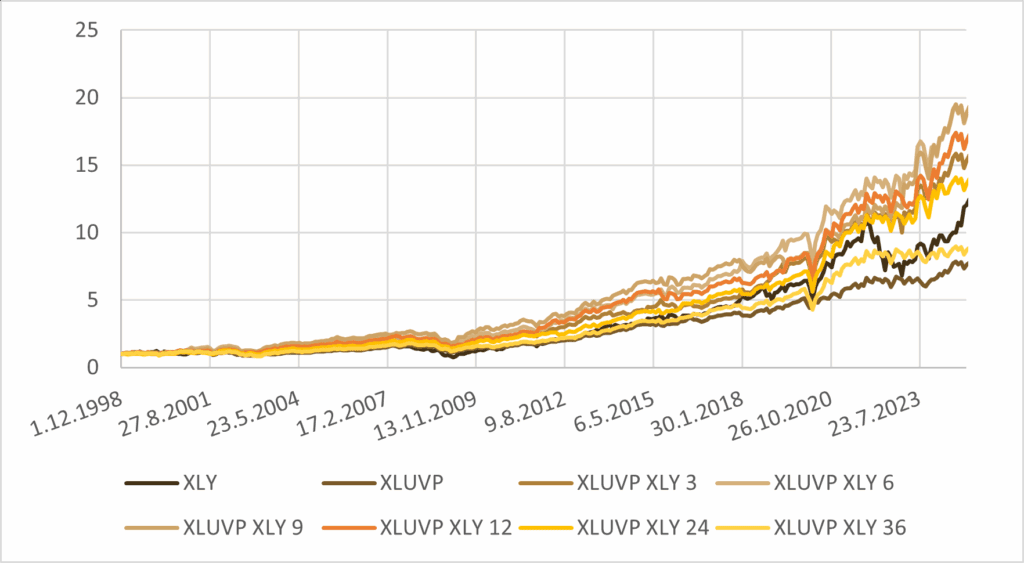
Table 4: Performance metrics of XLY – XLUVP switch strategies.
| PORTFOLIO | CAR p.a. | VOL p.a. | MAX DD | SHARPE | CALMAR |
|---|---|---|---|---|---|
| XLY portfolio | 9.70% | 19.24% | -54.93% | 0.5 | 0.18 |
| XLUVP portfolio | 7.96% | 11.38% | -33.45% | 0.70 | 0.24 |
| 3M XLY – XLUVP switch portfolio | 10.83% | 15.62% | -34.29% | 0.69 | 0.32 |
| 6M XLY – XLUVP switch portfolio | 11.67% | 15.77% | -36.79% | 0.74 | 0.32 |
| 9M XLY – XLUVP switch portfolio | 11.70% | 15.16% | -33.45% | 0.77 | 0.35 |
| 12M XLY – XLUVP switch portfolio | 11.21% | 14.27% | -35.14% | 0.79 | 0.32 |
| 24M XLY – XLUVP switch portfolio | 10.34% | 13.81% | -33.45% | 0.75 | 0.31 |
| 36M XLY – XLUVP switch portfolio | 8.50% | 13.06% | -33.45% | 0.65 | 0.25 |
The introduction of a defensive mix composed of XLP, XLU, and XLV has noticeably improved the performance metrics. We attribute this improvement to two factors. First, the combination of these three sectors inherently exhibits stronger risk-adjusted characteristics compared to any single component. Second, combining multiple defensive assets generally reduces overall portfolio risk, smoothing returns and lowering drawdowns.
Building on this principle, it is natural to extend the same multi-window aggregation approach that we previously applied to XLP alone. By averaging signals across different moving-average windows for the combined defensive portfolio, we aim to further reduce volatility and enhance stability. This allows the switch strategy to benefit simultaneously from both sector diversification and time-window diversification, potentially producing even more robust risk-adjusted outcomes.
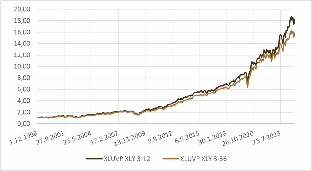
Table 5: Performance metrics of combining XLY – XLUVP switch strategies.
| PORTFOLIO | CAR p.a. | VOL p.a. | MAX DD | SHARPE | CALMAR |
|---|---|---|---|---|---|
| 3+6+9+12M XLY – XLUVP switch portfolio | 11.51% | 14.23% | -31.83% | 0.81 | 0.36 |
| 3+6+9+12+24+36M XLY – XLUVP switch portfolio | 10.93% | 13.11% | -31.43% | 0.83 | 035 |
Once again, the results confirm that the defensive mix of XLP, XLU, and XLV outperforms a portfolio using only XLP on the defensive side. The combination provides stronger risk-adjusted metrics, reduces drawdowns, and delivers a more stable return profile, demonstrating the benefits of both sector diversification and multi-window signal aggregation within the switch strategy.
Does this approach work for individual stocks as well?
A new question naturally arises from our sector-level results. The switch strategy works exceptionally well with sector ETFs, which is encouraging, but its utility could be further enhanced if it were applicable to selected individual stocks. To explore this, we turn our attention to Amazon (AMZN), one of the largest consumers of packaging materials tracked by our indicator. By applying the same multi-window, switch-based approach, we aim to investigate whether the strategy can capture similar risk-adjusted improvements and generate meaningful signals at the single-stock level.
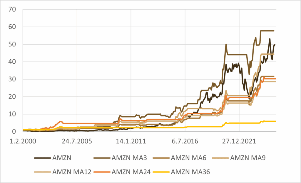
Table 6: Performance metrics of AMZN switch strategies.
| PORTFOLIO | CAR p.a. | VOL p.a. | MAX DD | SHARPE | CALMAR |
|---|---|---|---|---|---|
| AMZN portfolio | 20.72% | 38.79% | -86.04% | 0.53 | 0.24 |
| 3M AMZN switch portfolio | 21.67% | 27.81% | -60.75% | 0.78 | 0.36 |
| 6M AMZN switch portfolio | 18.18% | 26.52% | -64.72% | 0.69 | 0.28 |
| 9M AMZN switch portfolio | 20.14% | 26.57% | -52.66% | 0.76 | 0.38 |
| 12M AMZN switch portfolio | 17.61% | 22.89% | -51.40% | 0.77 | 0.34 |
| 24M AMZN switch portfolio | 17.94% | 18.00% | -22.72% | 1.00 | 0.79 |
| 36M AMZN switch portfolio | 9.01% | 12.95% | -19.40% | 0.70 | 0.46 |
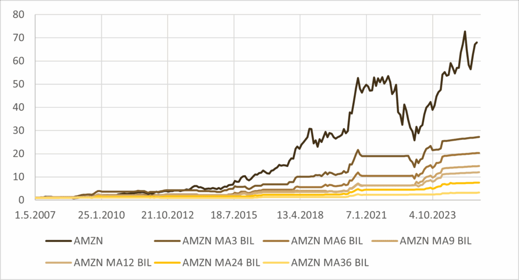
We observe that as we extend the moving-average window in the MA model, the raw returns tend to decline. While risk-adjusted metrics improve slightly, the reduction in absolute performance is a concern. Moreover, longer windows often result in prolonged periods of inactivity, during which the strategy simply holds no position. To address this, we consider integrating BIL, a short-term Treasury ETF, into the portfolio. By allocating idle cash to BIL, the strategy can generate at least modest returns during inactive periods, improving overall efficiency without materially increasing risk. This adjustment allows the model to remain conservative when signals are weak while still putting idle capital to productive use.
Changing the observation period led to a reduction in raw returns, but it also occasionally improved certain risk-adjusted metrics.
Table 7: Performance metrics of AMZN – BIL switch strategies.
| PORTFOLIO | CAR p.a. | VOL p.a. | MAX DD | SHARPE | CALMAR |
|---|---|---|---|---|---|
| AMZN portfolio | 25.64% | 39.15% | -51.92% | 0.65 | 0.49 |
| 3M AMZN – BIL switch portfolio | 19.68% | 21.24% | -34.10% | 0.93 | 0.58 |
| 6M AMZN – BIL switch portfolio | 17.80% | 20.66% | -22.52% | 0.86 | 0.79 |
| 9M AMZN – BIL switch portfolio | 15.73% | 19.30% | -31.57% | 0.81 | 0.50 |
| 12M AMZN – BIL switch portfolio | 14.46% | 17.54% | -29.63% | 0.82 | 0.49 |
| 24M AMZN – BIL switch portfolio | 11.60% | 14.25% | -19.58% | 0.81 | 0.59 |
| 36M AMZN – BIL switch portfolio | 6.57% | 10.06% | -12.01% | 0.65 | 0.55 |
We can also consider whether combining multiple window lengths adds value. To explore this, we revisit the mixed-horizon approach used earlier and test combinations of 3–12 month and 3–36 month MA-based strategies.
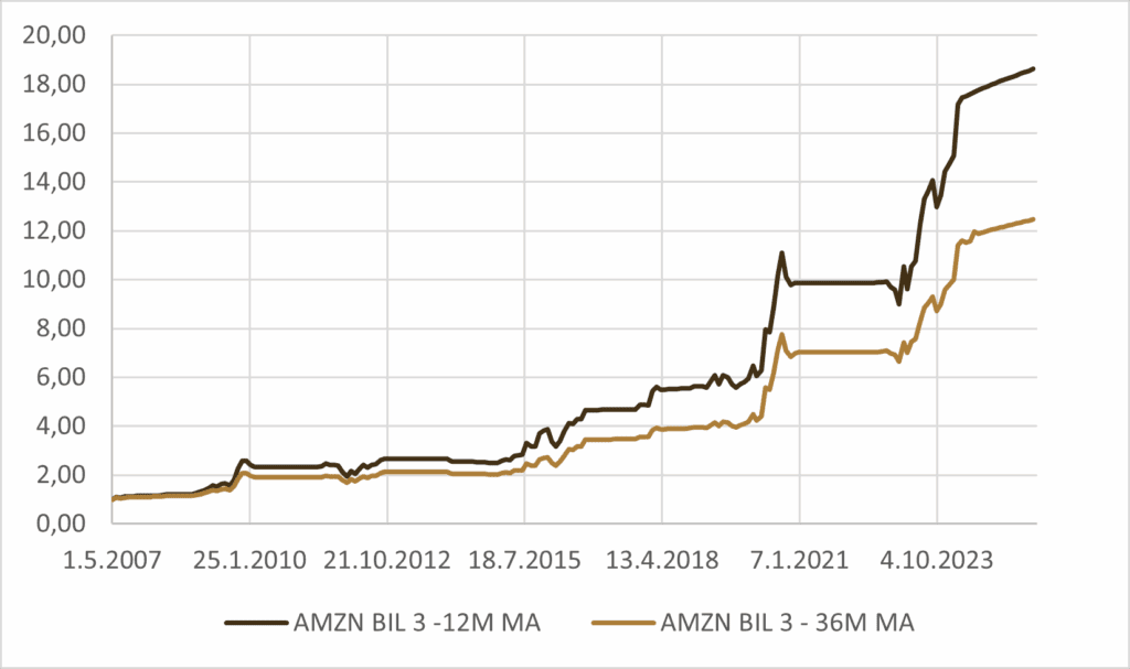
Table 8: Performance metrics of combining AMZN – BIL switch strategies.
| PORTFOLIO | CAR p.a. | VOL p.a. | MAX DD | SHARPE | CALMAR |
|---|---|---|---|---|---|
| 3+6+9+12M AMZN – BIL switch portfolio | 17.23% | 18.07% | -25.33% | 0.95 | 0.68 |
| 3+6+9+12+24+36M AMZN – BIL switch portfolio | 14.69% | 14.82% | -19.27% | 0.99 | 0.76 |
Once again, the results show that combining multiple signals produces a more stable and balanced outcome. The nominal return decreases, but the overall behavior of the strategy becomes more disciplined, less volatile and more resilient in difficult market periods. Blending different window lengths consistently improves risk-adjusted performance, which can be more valuable than purely maximizing raw returns.
Summary and conclusion
Over the course of our analysis, we experimented with a wide range of approaches built around the idea of using the corrugated-box PPI as an alternative market signal. We evaluated AR and MA models, different window lengths, single-indicator strategies and blended multi-window systems. The clearest conclusion is that this methodology works most naturally with sector ETFs, where the indicator provides a meaningful trigger for rotating between offensive assets such as XLY and defensive assets such as XLP, XLU or XLV. Sector-level dynamics react more visibly to changes in underlying economic activity, which makes the switching mechanism both intuitive and effective.
When applying the same logic to individual equities, the results were not as clean. The indicator does not translate as directly into firm-level behavior, which means that while nominal returns often decline, we can still achieve improvements in risk-adjusted metrics like Sharpe and Calmar. This comes at a noticeable cost in raw performance, but it demonstrates that the core idea retains some value even in a less favorable setting.
Finally, it is worth emphasizing that this PPI series is only one example within a much broader universe of alternative indicators. Many unconventional macro or micro-level metrics may carry predictive structure that traditional price-based signals fail to capture. Exploring these sources systematically can reveal new perspectives on market behavior and potentially uncover robust decision frameworks for active allocation.
Author:
David Belobrad, Junior Quant Analyst, Quantpedia
Are you looking for more strategies to read about? Sign up for our newsletter or visit our Blog or Screener.
Do you want to learn more about Quantpedia Premium service? Check how Quantpedia works, our mission and Premium pricing offer.
Do you want to learn more about Quantpedia Pro service? Check its description, watch videos, review reporting capabilities and visit our pricing offer.
Do you want algorithmic access to the full Quantpedia database via the API? Subscribe to Quantpedia Pro, ask for an API key, and explore the in/out-of-sample statistics, source academic papers, and code snippets — ideal for quantitative research, systematic trading workflows, and AI model training.
Are you looking for historical data or backtesting platforms? Check our list of Algo Trading Discounts.
Or follow us on:
Facebook Group, Facebook Page, Telegram, Twitter, Linkedin, Medium or Youtube
Share onLinkedInTwitterFacebookRefer to a friend


