Analysis of Price-Based Quantitative Strategies for Country Valuation
Introduction
Value investing originated as an investment strategy in which investors try to beat the stock market by looking for stocks that trade at a price below their intrinsic value or book value. Value investors do not subscribe to the efficient-market hypothesis, which suggests that stock prices always reflect their intrinsic value. Instead, value investors believe stocks can be overvalued or undervalued due to various factors. The market is believed to often overreact to news or events, leading to a gap between the stock price and the company’s long-term fundamentals. This overreaction creates an opportunity for value investors to buy stocks at a discount in the hope that the market will eventually recognize the stock’s true value, leading to an increase in price. By actively seeking out undervalued stocks, value investors aim to exploit the market’s tendency to misprice securities.
We would reiterate that value investing is truly a long-term strategy, and Warren Buffett is famous for his patient and long-term approach to it. He often buys stocks intending to hold them indefinitely, focusing on the value and long-term potential of the companies he invests in. Buffett’s quotes emphasize his commitment to the long-term nature of value investing, where he does not try to make quick profits in the stock market but instead looks for strong companies that he believes in. that will increase in value over time. By maintaining a diversified stock portfolio and maintaining a long-term perspective, investors can wait to sell their stocks until the price exceeds their fair market value and the price they set pay them, thereby maximizing potential profits. This approach is consistent with the idea of holding quality investments and selling only when the market recognizes their true value.
But value strategies are not used just in stocks. There are a lot of different definitions of “value” and the idea of buying “cheap assets” is in widespread use in currencies (Currency Value – PPP Factor), country ETFs (Value Factor – CAPE Effect within Countries), or in a diversified portfolio of assets in general (Value and Momentum Factors across Asset Classes).
If you are more interested in value investing, you might also find our two-part primer on what’s been working best lately interesting:
You are also welcome to explore other value strategies we provide in our Screener.
Approach, Methodology, and Motivation
The motivation for this study comes from the idea of simplifying the concept of relative valuation among the countries. There exist several ideas for relative value approaches that compare the “visible price” (or market capitalization) of the stock market to some unseen “intrinsic value” of the market. The ideas of what we can use to measure the unseen “intrinsic value” of each individual country/market are numerous – it may be a number derived from GDP (like in a Buffet Indicator), total earnings of listed companies in the selected country (Shiller’s CAPE ratio), or ratios derived from yields, demographic, etc., etc. All of those ratios use some non-price data in order to obtain an “intrinsic value” for each country. It has a lot of advantages (non-price measures can add a lot of important information for valuation models), but also some disadvantages (the biggest disadvantage is that we must have a source of high-quality data for those non-price data for all countries and additionally, data are often published with a significant lag). So we asked ourselves – can we create a relative valuation model and use just the price data?
How do we proceed? As we have mentioned before, non-price data (like growth in GDP or total earnings of all companies in the selected country) have the advantage of hidden information. On the other hand, those data usually do not change very often on a year-to-year (quarter-to-quarter) basis. The volatility of non-price data is significantly lower than the volatility of stock indices data alone. This also means that change in most of the relative valuation ratios like market value of equity (MVE) scaled by gross domestic product (GDP) (Buffet Indicator) or CAPE (Shiller’s Cyclically Adjusted Price to Earnings Ratio) is driven by the change in the nominator part of the ratio (price-related part) and not by a change in the denominator (non-price anchor), which rarely changes a lot. Suppose the denominator part is only a slow-moving anchor. In that case, we can easily omit using the non-price data, replace them with some average value calculated from the cross-section of price data from all countries, and proceed with the model trying to value countries among themselves by using just the price data. So, that’s the theory, but the question is – were we successful?
To summarize, our approach is simple and straightforward: naïve 20 country indices are averaged into the average country index with equal weight, and all countries with a long-term performance above average are taken as overvalued in that sense, and underperforming countries do qualify as undervalued.
We will test multiple different definitions for the country’s past outperformance and/or underperformance (using momentum, moving averages, and regressions), and optimal sorting, rebalancing horizons, and cut-off points (vigintiles, deciles, quintiles, quartiles, terciles, halves).
Data and Signals
We use monthly data, dividends, and split-adjusted. Yahoo Finance was chosen to collect data about ETFs from their inception. Then, we used the MSCI website to download missing country indices to enlarge the dataset to the maximum possible length. The following countries/ETFs were included in the analysis:
| ticker | full name |
| EWU | iShares MSCI United Kingdom ETF |
| EWG | iShares MSCI Germany ETF |
| EWQ | iShares MSCI France ETF |
| EWI | iShares MSCI Italy ETF |
| EWD | iShares MSCI Sweden ETF |
| EWN | iShares MSCI Netherlands ETF |
| EWP | iShares MSCI Spain ETF |
| EWK | iShares MSCI Belgium ETF |
| EWL | iShares MSCI Switzerland ETF |
| EWC | iShares MSCI Canada ETF |
| EWJ | iShares MSCI Japan ETF |
| EWW | iShares MSCI Mexico ETF |
| EWM | iShares MSCI Malaysia ETF |
| EWA | iShares MSCI-Australia ETF |
| EWS | iShares MSCI Singapore ETF |
| EWY | iShares MSCI South Korea ETF |
| EWT | iShares MSCI Taiwan ETF |
| EWZ | iShares MSCI Brazil ETF |
| EZA | iShares MSCI South Africa ETF |
| FXI | iShares China Large-Cap ETF |
| INDY | iShares India 50 ETF |
We have decided not to include the U.S. (United States) since we focus on ex-U. S. World. United States is around 50 % of the global market cap; therefore, it would make better sense to make a model that evaluates the U.S. vs. the rest of the world and not just include the U.S. market in the sample. However, the model for relative valuation of the U.S. market vs. the rest of the world is not the primary aspect and goal of this study (we will get to that in some future articles).
The proportion between World and U. S. is shown in the following figure:

We leave the first five years of data (from 1992-12-31 to 1997-12-31) only for calculations (we call it the “calculation period”) and, therefore, our equity curves start five years after that. The ending date we consider data up to is 2023-03-31. Most country ETFs started trading on 1996-04-01 and, upon that date, were enriched by indices values from 1992-12-31, the common denominator for all countries considered. These came from global, regional, or country MSCI index websites. We select the Standard (Large+Mid Cap) Size of the index for them, all in USD Currency.
Recently, Yahoo Finance discontinued free end-of-day data downloads. As a result, we recommend sourcing data from our preferred provider, EODHD.com – the sponsor of our blog. EODHD offers seamless access to +30 years of historical prices and fundamental data for stocks, ETFs, forex, and cryptocurrencies across 60+ exchanges, available via API or no-code add-ons for Excel and Google Sheets. As a special offer, our blog readers can enjoy an exclusive 30% discount on premium EODHD plans.
Holding Periods and Execution Techniques
Since it is a valuation signal, we deliberately chose a longer period and initially considered 3 of them (they were developed on an ad hoc basis and from our best guesstimates):
- 4x tranche, 12-month holding period (1 year), quarterly re-balancing,
- 12x tranche, 36-month holding period (3 years), quarterly re-balancing,
- 10x tranche, 60-month holding period (5 years), half-year re-balancing.
Quarterly rebalancing is, for example, done 31.12, 31.3, 30.6, and 30.9 each year. For the execution method, we use an industry-standard tranching application, meaning we will always re-balance only the pre-selected part of the portfolio.
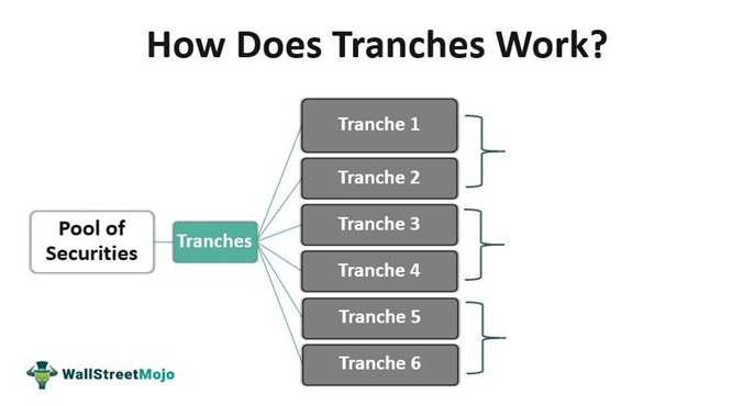
We divide the portfolio into 12 sub-portfolios; each part would be rebalanced once per 3 years and would be weighted as 1/12 from weight in full (total; final) portfolio.
So, explained:
31.12.1997 is being invested first 1/12; we select 25% overbought and go short them, and a 25% oversold, which we go long and hold until 31.12.2000 when we re-balance again for a 3-year holding period.
The same was done for 31.3.1998, which was held until 31.3.2001, and then again from 1999 to 2002; that is, the tranching for 12 quasi-sub-strategies / tranches. The final portfolio is equally weighted among these 12.
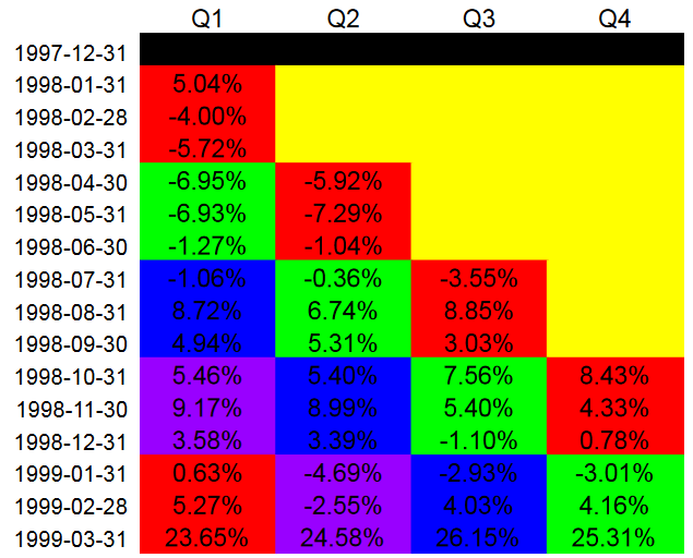
And here is the example mentioned depicted as performed on four tranches each month:
Price-Based Valuation Signals
We have considered three basic principles to apply to our suited solution:
- Price vs. MA (moving average) — this is a strategy traded as a reversal (mean reverting signal); that is: we go long (buy) countries where price is lowest compared to their 60-month MA and go short (sell short) countries where prices are highest against 60-month MA.
- Past Momentum signal — this strategy is also traded as a reversal (mean reverting signal); we go long countries with the worst 60-month momentum and short (sell short) countries with the best 60-month momentum.
- Linear regression – Wikipedia article states that simple linear regression is a linear regression model with a single explanatory variable with one independent variable and one dependent variable. (Simple) Linear Regression, y=α + β*x, which has usual parameters:
- (regression) slope — β;
- (regression) intercept — axes-intercept α; that describes a linear line y.
- We use both α as our valuation predictor
SLR ([Simple] Linear Regression)
Here is a bit of a detailed description of strategies that use regression approach:
- We do a regression of each country against the equal-weighted averaged index explained before; we use rolling five years window for regression calculations.
- Y variable is the monthly return of the individual country,
- and X is the monthly performance of the equal-weighted averaged index
- We calculate slope β and intercept α for each country every month.
- We long (buy) the lowest alpha and short (sell) the highest alpha countries
- Calculate all performance metrics and evaluate.
Number of ETFs in a portfolio
- 1 ETF long vs. 1 ETF short (vigintiles),
- 2 vs. 2 (deciles),
- 3 vs 3,
- 4 vs 4 (quintiles),
- 5 vs 5 (quartiles),
- 7 vs 7 (terciles),
- 11 vs 11 (halves).
Main Results
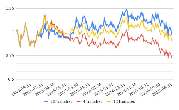
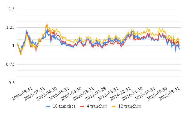
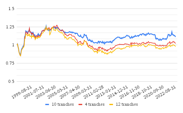
1.The impact of the number of ETFs in a portfolio – Price vs. MA signal
The move from vigintile (1 ETF vs. 1 ETF) and decile (2 vs. 2) to tercile (7 vs. 7) and a half (11 ETFs vs. 11 ETFs) decreases volatility gradually since the portfolio is more diversified. It’s not the case for all of the strategy variants, but in the case of Price vs. MA signal, performance is improving too.
We can see this effect at all tested variants of for the Price vs. MA signal, The following charts show this diversification effect going from 1vs1 portfolio to 11vs11 portfolio:
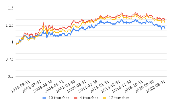
The subsequent table show the performance and risk ratios of the most diversified (11vs11) variant of the country ETF long/short strategy.
| tranche | CAR p.a. | Volatility p.a. | Sharpe Ratio | Max DD | CAR / max DD |
|---|---|---|---|---|---|
| 4x | 1.14% | 3.92% | 0.29 | -9.85% | 0.12 |
| 12x | 1.04% | 3.85% | 0.27 | -8.55% | 0.12 |
| 10x | 0.78% | 3.69% | 0.21 | -9.80% | 0.08 |
The strategy has a low volatility but also low total performance. The low performance of the strategy shows that there is not a lot of value factor alpha that can be captured in the cross-section of the country ETFs. This finding is consistent with the recent research paper from Audrey Dong, Mia Huang, and Mamdouh Medhat, which reports similar results. It seems that the countries’ ETF market is quite efficient, and it’s better to try to capture the alpha on the security level.
Also, most of the alpha is incurred until 2015; afterward, the equity curves are mostly flat. This is consistent with the other effect – the general tendency of value strategies to underperform in the last decade. It seems that value strategy in country ETFs is not an exception.
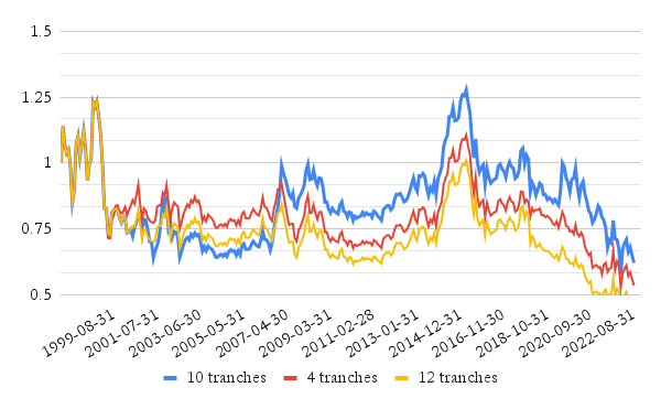
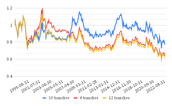
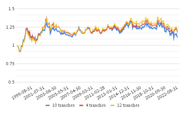
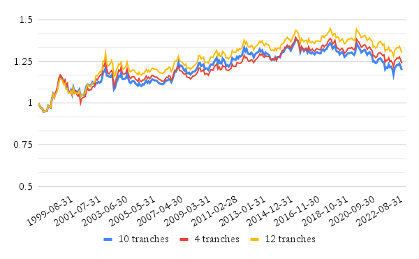
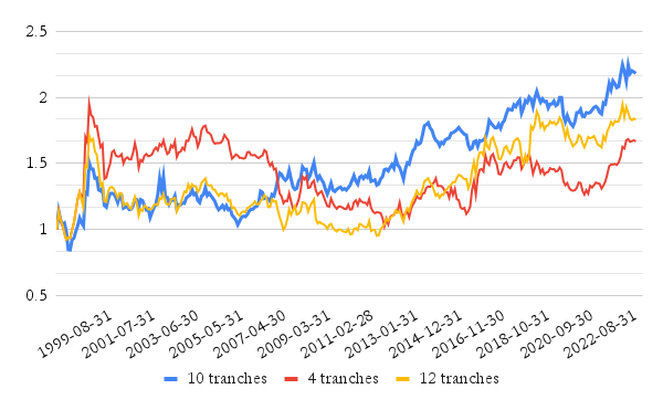
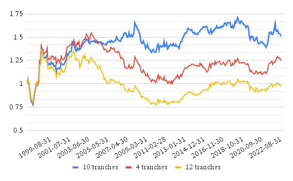
2.The impact of the number of ETFs in a portfolio – Intercept signal
The second main finding is related to the Intercept strategy. Just for recapitulation – in this variant of the country value strategy, we go long the country ETFs with the lowest alpha (regression intercept) against the equal-weighted averaged index, and we go short the coutnry ETFs with the highest alpha regression intercept) against the equal-weighted averaged index. Once again, following charts show diversification effect going from 1vs1 portfolio to 11vs11 portfolio:
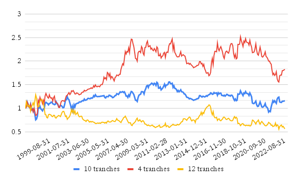
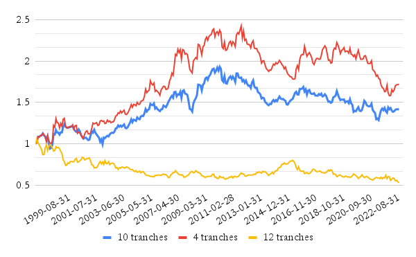
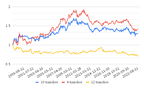
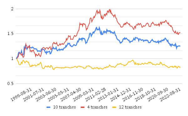
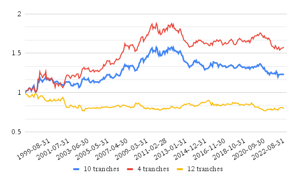
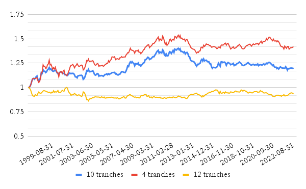
We can see that the Intercept signal works well for 12-month (4 tranches, quarterly rebalanced portfolio) and 60-month holding periods (10 tranches, half-year rebalancing) but not very well for 36-month holding period (12-tranches, quarterly rebalancing). When we compare risk and return ratios, we see that the return of the “betting-against-alpha” value strategy is best when our portfolio is the least diversified, but the Sharpe ratio is the lowest. As we diversify our portfolio among more ETFs, total performance decreases, but Sharpe ratio and CAR/maxDD ratios increase as in the case of Price vs. MA signal.
Overall, the “betting-against-alpha” value strategy in the country ETF space has similar characteristics as the previous Price vs. MA strategy – relatively good performance until the year 2013 and flat equity curves afterward. It seems that we are also not able to escape the curse of the value factor in this case…
| version | CAR p.a. | Volatility p.a. | Sharpe Ratio | Max DD | CAR / max DD |
|---|---|---|---|---|---|
| 1v1 | 2.39% | 14.78% | 0.16 | -38.05% | 0.06 |
| 2v2 | 2.16% | 10.18% | 0.21 | -34.64% | 0.06 |
| 3v3 | 1.35% | 8.42% | 0.16 | -32.63% | 0.04 |
| 4v4 | 1.37% | 8.02% | 0.17 | -28.82% | 0.05 |
| 5v5 | 1.69% | 7.38% | 0.23 | -25.24% | 0.07 |
| 7v7 | 1.80% | 6.39% | 0.28 | -17.98% | 0.10 |
| 11v11 | 1.38% | 4.62% | 0.30 | -13.33% | 0.10 |
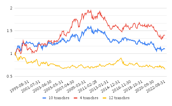
We use the momentum signal opposite to trend-following strategies. Our value (mean-reversion) strategy buys the past 60-month momentum losers and sells the winners. What are the results? It’s the weakest signal for the relative country valuation strategy if we compare it to the previous valuation models. We only show a few charts, not all variants of the strategy. But from the charts, we can see that an undiversified strategy produces some return (albeit very volatile). As we diversify our portfolio, the performance of the strategy goes to zero.
Discussion
Indeed, we have undergone an interesting thought process, but it did not yield the expected results. Unfortunately, it seems that explanatory and statistical power is lower than we wanted to achieve, and price-only valuation signals are weaker than relative valuation signals that use non-price signal variables such as CAPE, MVE vs. GDP, etc.
It also seems that despite the significant number of country ETFs, this market segment is quite efficient. Additionally, it’s even harder to find a reliable long/short value strategy that has performed well in the last ten years when all of the other value strategies also struggled. But there is one positive outcome out of all of it – that we satisfied our curiosity and can move to the next challenge 🙂
Are you looking for more strategies to read about? Sign up for our newsletter or visit our Blog or Screener.
Do you want to learn more about Quantpedia Premium service? Check how Quantpedia works, our mission and Premium pricing offer.
Do you want to learn more about Quantpedia Pro service? Check its description, watch videos, review reporting capabilities and visit our pricing offer.
Do you want algorithmic access to the full Quantpedia database via the API? Subscribe to Quantpedia Pro, ask for an API key, and explore the in/out-of-sample statistics, source academic papers, and code snippets — ideal for quantitative research, systematic trading workflows, and AI model training.
Are you looking for historical data or backtesting platforms? Check our list of Algo Trading Discounts.
Or follow us on:
Facebook Group, Facebook Page, Telegram, Twitter, Linkedin, Medium or Youtube
Share onLinkedInTwitterFacebookRefer to a friend


