A new financial research paper gives an ideas of how to allocate capital across several well known factor strategies:

Authors: Blin, Ielpo, Lee, Teiletche

Title: Factor Timing Revisited: Alternative Risk Premia Allocation Based on Nowcasting and Valuation Signals

Link: https://papers.ssrn.com/sol3/papers.cfm?abstract_id=3247010

Abstract:

Alternative risk premia are encountering growing interest from investors. The vast majority of the academic literature has been focusing on describing the alternative risk premia (typically, momentum, carry and value strategies) individually. In this article, we investigate the question of allocation across a diversified range of cross-asset alternative risk premia over the period 1990-2018. For this, we design an active (macro risk-based) allocation framework that notably aims to exploit alternative risk premia’s varying behavior in different macro regimes and their valuations over time. We perform backtests of the allocation strategy in an out-of-sample setting, shedding light on the significance of both sources of information.

Notable quotations from the academic research paper:

"Alternative risk premia investing has grown rapidly in popularity in the investment community in recent years. They provide systematic exposures to risk factors and market anomalies that have frequently been widely analyzed in academic research. The vast majority of the academic literature solely focuses on the identification and the analysis of individual alternative risk premia strategies. On the contrary, this article addresses the question of allocation among alternative risk premia.

The standard approach in the industry is to apply a risk-based allocation mechanism, particularly equal risk contribution (ERC) in which one allocates the same risk budget to all components in the portfolio. One of the perceived key benefits of this approach is that it does not require expected returns as input but solely risk measures, hence the name “risk-based”. This no-views/agnostic feature alleviates the pitfalls of forecasting, which is already a challenge for traditional assets but even more so for alternative risk premia that are newer or are perceived as more complex strategies.

Despite this, recent research lends more support to the idea of some predictability of factor returns. In this article, we extend those results by focusing on the relationship between alternative risk premia and macro regimes that we define through nowcaster indicators. We consider that three major macroeconomic risks that affect risk premia: growth, inflation and market stress/volatility.

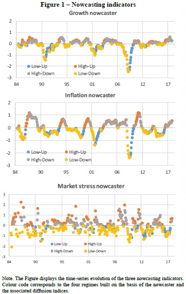
To model the influence of these macro risks, a regime approach has proven effective. To characterize macro regimes for growth, inflation and market stress, we build our own nowcasting (contraction of “now” and “forecasting”) indicators since 1990. Seeking for simplicity, our nowcasters are simple averages of z-scores of a large cross section of indicators across a large set of countries. For instance, the “growth” nowcaster contains close to 500 economic times-series across major developed and emerging countries accounting for 85% of world GDP. In Appendix A, we provide more details on the construction of the nowcasters.

To characterize economic regimes in a more precise way, we use both the average of all properly scaled economic indicators (the “nowcaster” per se) but also take advantage of the information in the cross-section by accounting for the proportion of indicators that are improving or deteriorating for every period (called “diffusion” index below). In practice, the diffusion index gives some further indication about whether the economy is improving (when diffusion index rises) or deteriorating (when diffusion index declines). On the basis of the nowcaster and diffusion indices, we define four regimes:

– Low-Up: negative nowcaster (Low) and diffusion index above 50% (Up)
– Low-Down: negative nowcaster (Low) and diffusion index below 50% (Down)
– High-Up: positive nowcaster (High) and diffusion index above 50% (Up)
– High-Down: positive nowcaster (High) and diffusion index below 50% (Down)

For the growth factor, this is similar to the usual Recession (Low-Down) / Recovery (Low-Up) / Expansion (High-Up) / Slowdown (High-Down) classification.

In Figure 1, we represent the different macro factor nowcasters and highlight different regimes by using a distinctive color scheme.

To give a first sense of the sensitivity of alternative risk premia to macroeconomic regimes, we represent in Figure 2 growth regime-conditional excess Sharpe ratios, i.e. the difference between Sharpe ratios in each growth regime and the long-term (unconditional) Sharpe ratio. Some strategies can be seen as being “defensive”, as they tend to do relatively well in either slowdowns (High-Down regime) or recessions (Low-Down regime), such as equity quality, equity low-risk, trend-following, or bonds carry. Conversely, some strategies benefits from better economic conditions such as equity size, FX carry or volatility carry.

In next section, we define and implement a process to allocate among alternative risk premia which incorporates, along other dimensions, each risk premium’s sensitivities to the macro regimes. The approach is based on the active risk-based methodology derived in Jurczenko and Teiletche (2018) which adapts Black and Litterman (1992) framework to the risk-based world. In practice, the model ends up combining a risk-based strategic portfolio with a set of dynamic allocation active views.

As our focus is on dynamic signals, we do not seek to improve the strategic portfolio. We adopt a simple ERC portfolio, which consists of equal contributions to portfolio volatility across all alternative risk premia. The strategic portfolio is then modified to incorporate dynamic deviations in two steps.

In a first step, we compute z-score reflecting dynamic allocation based on an equal-weight of two z-scores, for macro factors and valuation respectively. Regarding macro factors (growth, inflation, market stress), z-scores are computed as the excess return in the current (“nowcasted”) regime vs full sample return scaled by historical volatility.

In the second step, these dynamic z-scores are transformed into active portfolio deviations calibrated to deliver 1% tracking-error relative to the strategic portfolio. The sum of active deviations is set to zero, so that the portfolio is fully invested, similar to the strategic allocation.

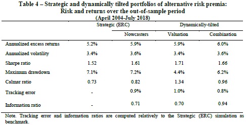
Table 4 summarizes the performance statistics of the portfolio. The first column shows the strategic ERC portfolio. The second to fourth columns show the “dynamic” portfolios that incorporate active tilts, based on nowcasters and valuation signals individually and in combination.

"

Are you looking for more strategies to read about? Check http://quantpedia.com/Screener

Do you want to see an overview of our database of trading strategies? Check https://quantpedia.com/Chart

Do you want to know how we are searching new strategies? Check https://quantpedia.com/Home/How

Do you want to know more about us? Check http://quantpedia.com/Home/About

Follow us on:

Facebook: https://www.facebook.com/quantpedia/

Twitter: https://twitter.com/quantpedia

A new financial research paper has been published and is related to all equity long short strategies but mainly to:

#33 – Post-Earnings Announcement Effect

Authors: Li

Title: Does Too Much Arbitrage Destablize Stock Price? Evidence from Short Selling and Post Earnings Announcement Drift.

Link: https://papers.ssrn.com/sol3/papers.cfm?abstract_id=3249254

Abstract:

Stein (2009) suggests that too much arbitrage capital exploiting underreaction can lead to overreaction, pushing price further away from fundamental value. I test this hypothesis by investigating the relation between changes in short interest ratio around earning announcement and the subsequent drift return. There are two main findings in this paper. First, my results suggest that too much arbitrage capital does contribute to overreaction (with a t-statistics around 4 on average). These findings are robust to alternative sample periods or length of the window for drift calculation. Second, contrary to the findings in prior literature that show that short sellers mitigate the magnitude of drift, my results show that almost all of this effect are actually contributed by the observations that are more likely to represent overreaction.

Notable quotations from the academic research paper:

"Conventional wisdom believes that as more arbitrage capital starts to trade a given anomaly, any abnormal returns will be eventually eliminated (up to risk and limits to arbitrage) and stock prices will be pushed closer to fundamental values. In other words, the more arbitrage capital, the more efficient the market is likely to become. However, Stein (2009, Presidential Address: Sophisticated Investors and Market Efficiency) questions this simple intuition and shows that when the anomaly does not have a fundamental anchor and when arbitrageurs are not aware about how many other arbitrageurs are trading the same anomaly, arbitrage activity may lead to price overshoot, pushing price further away from fundamental value. Prior literature has very little empirical evidence regarding this implication. Therefore, in this study I try to test whether too much arbitrage capital destabilizes stock price.

The anomaly utilized in this paper is post earnings announcement drift (henceforth, PEAD). Three major advantages associated with PEAD makes it an ideal setting for testing the above implication.

First, it does not have a fundamental anchor so that arbitrageurs do not have a benchmark to gauge the level of under or over valuation. Second, it is one of the most persistent anomalies that are often followed by actively managed hedge funds. Third, it allows me to pin down the time at which arbitrageurs are most likely to take actions – that is, if an arbitrageur was to maximize his profit, he would be more likely to take action in a tight window around the earnings announcement date.

The proxy for arbitrage capital is the change of short interest ratio around earnings announcement date. It is widely documented that short sellers tend to be informed traders who incorporate information and move prices closer to fundamental values. Also note that, in this study, I only focus on announcements with negative earnings surprise since these are the stocks that short sellers are more likely to target.

The relation between PEAD and change of short interest ratio is illustrated in figure 1.

Day 0 is the date when the earning announcement is released. Day -1 is one day before and Day 1 is one day after the announcement date. Together, the 3-day window forms the initial response period in which arbitrageurs will trade most intensively. The solid line illustrates the return pattern for negative earnings surprise announcement with insufficient arbitrage capital. In this case, a minor negative return is realized in the initial response period which is followed by a further negative drift. The dashed line illustrates the case when there is sufficient arbitrage capital. In this case, more arbitrage capital adjusts the price to fundamental value faster and therefore a moderate negative return (more negative than the solid line) is realized and no obvious further drift follows. The crossed line illustrates the case when there is too much arbitrage capital. In this case, due to too much arbitraging, a large negative initial response (potential overshoot) is followed by a positive drift (correction).

My findings suggest that too much arbitrage does seem to destabilize stock price. First, holding all else equal, announcements with larger increase in short interest ratio experience significantly more negative initial response (more correction). Next, I show that negative earnings announcements with positive abnormal drift have significantly higher change in short interest ratio than those with negative abnormal drift. Moreover, I find that, holding all else equal, stocks with the largest increase in short interest ratio (SIR decile 10) is almost 10% more likely to result in overreaction than stocks with the largest decrease in short interest ratio (SIR decile 1). In the end, I show that, holding all else equal, change in short interest ratio significantly contributes to overreaction. In particular, within stocks that have positive abnormal drift, the ones that experience the largest increase in short interest ratio average 1.55% higher drift than the ones that experience the largest decrease in short interest ratio. Robustness tests show that my results are not likely to be driven by extreme values in abnormal drift, particular year observations, or length of window for return calculations."

Are you looking for more strategies to read about? Check http://quantpedia.com/Screener

Do you want to see an overview of our database of trading strategies? Check https://quantpedia.com/Chart

Do you want to know how we are searching new strategies? Check https://quantpedia.com/Home/How

Do you want to know more about us? Check http://quantpedia.com/Home/About

Follow us on:

Facebook: https://www.facebook.com/quantpedia/

Twitter: https://twitter.com/quantpedia

We have mentioned it several times – we are quants but we love history and we love research papers like this:

Author: McQuarrie

Title: The First Eighty Years of the US Bond Market: Investor Total Return from 1793, Combining Federal, Municipal, and Corporate Bonds

Link: https://papers.ssrn.com/sol3/papers.cfm?abstract_id=3260733

Abstract:

US securities markets took root after Alexander Hamilton’s refunding of the Federal debt in the early 1790s. Accordingly, a market in bonds has been in operation in the US for over two centuries. Until recently, however, little was known about the bond market prior to 1857. This paper focuses on investor holding period returns, using newly compiled data on bond prices, rather than focusing on the movement of yields, as in Homer (1963). It incorporates the relatively familiar Treasury securities from before President Andrew Jackson paid off the debt in 1835, but also includes state and city debt, which ballooned beginning in the 1820s, as well as corporate debt, from its beginnings about 1830 to its explosion after 1850. I find that all three classes of bonds provided investors with similar total returns, excepting a brief period in the 1840s when state securities plunged before recovering. I also find that real returns in the eight decades following 1793 were generally higher than the long-term average return of 3.6% proposed for bonds in Siegel (2014). I further find that in these early years, bonds sometimes out-performed stocks over periods of several decades, again contrary to Siegel’s thesis. The paper considers the implications of a demonstration that stocks and bonds performed differently in the nineteenth century as compared to the twentieth century.

Notable quotations from the academic research paper:

"The importance of the nineteenth century, in the context of financial history, is to provide a check on hasty generalizations from limited data. Returns from a few decades in the twentieth century, first made available in Fisher and Lorie (1964), must be regarded as limited indeed. This limited twentieth century data, which emerged as financial history was developing as a discipline and has been widely diffused in publications by Ibbotson (2016, Stocks, Bonds, Bills & Inflation), has strongly inflected conclusions about what investors can expect over the long-term. The twentieth century US data, especially following WW II when the US economy bestrode the world as a colossus, paints a very sunny picture for stocks, and a sad cloudy picture for bonds, memorialized in Siegel (2014, Stocks for the Long Run).

The US had a rather different economy in the nineteenth century, especially the antebellum years which have been the focus of this paper. Likewise, the US economy then held a very different and much more minor position in the world economy. Hence, it was rhetorically powerful for Siegel (2014) to advertise that two centuries of data told one consistent story: stocks are splendid, bonds are laggards. Consistent performance across two such wildly different epochs was strongly supportive of his thesis.

It now appears that Siegel’s (2014, Stocks for the Long Run) early nineteenth century database was both thinner than many readers may have realized (e.g., dividend payments were estimated rather than observed; many prominent stocks were excluded), and more prejudicial to bonds than may have been grasped (e.g., by taking the minimum of Federal and municipal yields, even after Federal bonds gained circulation privileges). The much thicker datasets here do not support Siegel’s attempt to generalize from mid-twentieth results to the very different circumstances faced by US investors in the early nineteenth century. As it becomes possible to stitch together an unbroken multi-century record for both stocks and bonds, discussion may turn to the factors that determine when stocks (bonds) will do well, and when stocks (bonds) will do poorly. There is now a counter to Siegel’s thesis: that both investments follow a random walk within bounds, and that these bounds may not differ by much across these two major categories of investment.

Stocks did out-perform bonds in the middle of the twentieth century, per Ibbotson and Siegel; but stocks did not out-perform bonds in the first few decades of the nineteenth century. Generalizations from the middle of the twentieth century do not hold—these now appear as simple extrapolations. Gainsaid in the nineteenth century, these extrapolated returns may not apply to the twenty-first century either.

Examining Figure 1, the pattern is straightforward. Yields rose through the 1790s, then declined until the War of 1812 (prior to the war, the government steadily paid down its debt). After the war Federal yields resumed their decline, ending at their low point for the period charted.

A simple summary of the newly uncovered sixty-four years of bond returns charted in Figure 12 might state:
1) returns for the period were well above the long-term average cited by Siegel (2014);
2) bonds are as subject to bull and bear markets as stocks;
3) bond returns can be depressed or super-charged over periods decades in length.

The most straightforward interpretation of Figure 14 is that bond investors never received the average return over any lengthy period. Rather, from time to time bond investors suffered depressed returns, most notably from the 1940s through 1980, but also from 1793 through 1814, while at other times, bond investors enjoyed sustained periods of unusually high returns, most notably from the end of the Civil War to the beginning of World War I, but also from the end of the War of 1812 to the beginning of the Civil War, and from 1981 to the present day. Bond investors were also vulnerable to sudden sharp shocks in which the real value of a bond portfolio dropped 30% or even 40% over a few years (these were mostly associated with bouts of wartime inflation). Conversely, during favorable periods bond investors could rack up multi-decade returns comparable to those expected from stocks. Over the eighty-seven years beginning in 1814, bond investors received an annualized real return of 7.12%–somewhat higher than the long-term return to be expected from stocks, according to Siegel, of 6.6%.

Figure 15 combines fifty years of bond data gathered in this paper with fifty years of stock returns. The pattern is not supportive of Siegel’s claim that stocks must out-perform bonds over decades-long periods. Nor does the pattern support Siegel’s (and Bernstein’s) expectation that real stock returns, measured over the long-term, will converge on an underlying constant, currently estimated by Siegel as 6.6%. Rather, stocks significantly underperformed this standard over the 1793-1843 period.

If Siegel (2014) had never published his thesis about stocks for the long run, and Figure 15 were the only evidence available on historical stock and bond returns in the nineteenth century, what would be the most straightforward interpretation of it?

Answer: that over most periods decades in length, stocks and bonds return about the same. Second, that returns fluctuate, consistent with a random walk within bounds, in which strings of good or bad performance, of any length, may occur. Accordingly, in the fullness of time sharp drops may occur, and stocks and bonds may drop together or not. Likewise, stocks and bonds may register an above-trend performance, lasting decades, which may be coincident or not. If the analyst is free to select an arbitrary beginning point, subject only to that point being decades in the past, then when measured at exactly the right (wrong) time, stocks can be shown to have under-performed bonds “over the long run.” The fifty years from 1793 provide such an example. Stocks returned 3.96% real annualized, while bonds returned 4.88%. As before, the difference sounds small until converted into ending portfolio values. Over those fifty years, perhaps one of the worst five-decade periods in the history of the US securities markets, stocks turned an investment of $1000 into $6,963, but bonds turned that $1000 into $10,807."

Are you looking for more strategies to read about? Check http://quantpedia.com/Screener

Do you want to see performance of trading systems we described? Check http://quantpedia.com/Chart/Performance

Do you want to know more about us? Check http://quantpedia.com/Home/About

Follow us on:

Facebook: https://www.facebook.com/quantpedia/

Twitter: https://twitter.com/quantpedia

Do you invest in emerging market bonds? A new interesting academic research paper just for you:

Author: Kang, So, Tziortziotis

Title: Embedded Betas and Better Bets: Factor Investing in Emerging Market Bonds

Link: https://papers.ssrn.com/sol3/papers.cfm?abstract_id=3196018

Abstract:

We document novel empirical insights driving the prices of sovereign external emerging market bonds. In the time series, we examine the market portfolio’s time-varying exposures to a broad set of macro factors (rates, credit, currency, and equity) and identify these embedded betas as key drivers of its excess returns. In the cross-section, we construct complementary value and momentum style factors and demonstrate their ability to explain country expected returns. Building off these insights, we introduce a simple risk-on versus risk-off framework to characterize the correlation structure spanning our macro and style factors. Lastly, we show how our style factors can be incorporated in an optimized long-only portfolio to generate outperformance relative to a value-weighted benchmark portfolio.

Notable quotations from the academic research paper:

"Our paper attempts to answer several salient questions:

What broad insights can macro factors provide into the time series of returns?

What country-specific insights can style factors provide into the cross-section of expected returns?

How can a factor-based investor systematically leverage these insights?

To motivate our paper, we begin by illustrating how macro factors have been a significant source of time-varying risk in the EMB universe. The top panel of Figure 1 decomposes the total risk of a value-weighted EMB portfolio between 2000 and 2017 in terms of macro risk factors. As expected, interest rate and credit risk factors appear to be the primary sources of risk, with relative risk contributions of 16% and 27%, respectively.2 While the EMB universe only includes USD denominated bonds with no explicit exposure to exchange rate fluctuations or global equity markets, our EM currency and global equity factors surprisingly account for 18% and 9% of the portfolio’s risk, respectively. Moreover, the bottom panel of Figure 1 reveals that these relative risk contributions have not been static, but in fact varied significantly over time.

Given these observations, our empirical analysis begins with an examination of the time series relationship between macro factors and EMB returns. We first highlight the impressive performance of the EMB portfolio, which realized an annualized excess return of 7.5% with a volatility of 9.0% over this sample period, corresponding to a Sharpe Ratio of 0.83. After controlling for its macro factor exposures, however, we find that the EMB portfolio realized no significant outperformance. We then examine the EMB portfolio’s macro factor exposures, which we call embedded betas, finding the relative risk contributions from these macro factors to be well balanced on average.

Next, we investigate the ability of value and momentum style factors to explain the cross section of country expected returns. We find that our risk-seeking value factor serves as an important source of risk-adjusted returns, while our momentum factor provides valuable defensive protection. We construct our value factor based on a measure we call default-adjusted spread, which corresponds to option-adjusted spread adjusted for expected sovereign default risk. On the other hand, our momentum factor exploits a simple cross-asset insight from currency markets to identify challenging sovereign credit conditions. Since a depreciating currency weakens a sovereign issuer’s ability to service its external debt, we argue that negative currency momentum should forecast lower bond prices to the extent that bond markets underreact to movements in the foreign exchange market.

Finally, we empirically test how incorporating our style factors in a long-only portfolio can generate outperformance relative to the value-weighted EMB portfolio through improved country selection bets. We do so by constructing and backtesting optimized long-only portfolios that incorporate realistic benchmark-relative constraints and trading frictions. We find that a multifactor strategy that combines value and momentum insights outperforms its value-weighted benchmark by 60 basis points per annum net of transaction costs, resulting in a net information ratio of 0.82."

Are you looking for more strategies to read about? Check http://quantpedia.com/Screener

Do you want to see performance of trading systems we described? Check http://quantpedia.com/Chart/Performance

Do you want to know more about us? Check http://quantpedia.com/Home/About

Follow us on:

Facebook: https://www.facebook.com/quantpedia/

Twitter: https://twitter.com/quantpedia

A new financial research paper has been published and is related to:

#77 – Beta Factor in Stocks

Authors: Liu

Title: Asset Pricing Anomalies and the Low-Risk Puzzle

Link: https://papers.ssrn.com/sol3/papers.cfm?abstract_id=3258015

Abstract:

The original observation in Black, Jensen and Scholes (1972) that the security market line is too flat – the beta anomaly – is a driving force behind a number of well-documented cross-sectional asset pricing puzzles. I document that returns to a broad set of anomaly portfolios are negatively correlated with the contemporaneous market excess return. I show that this negative covariance implicitly embeds the beta anomaly in these cross-sectional return puzzles. Taking into account the exposure to the beta anomaly either attenuates or eliminates the economic and statistical significance of the risk-adjusted returns to a large set of asset pricing anomalies.

Notable quotations from the academic research paper:

"Defying both theory and intuition, low beta assets have consistently outperformed high beta assets, both over time and across various asset markets. This observation has come to be known as the beta anomaly. In this paper, I present evidence that the beta anomaly is embedded in a broad set of cross-sectional asset pricing puzzles.

I document that anomaly portfolio returns share a striking and peculiar pattern: returns are positive and peak in market downfalls, but are negative when the market rises. I verify that this negative covariance is empirically equivalent to the long portfolios holding stocks with lower betas relative to the short portfolios. Mitigating the exposure to the beta anomaly either attenuates or eliminates the economic and statistical significance of the risk-adjusted returns to numerous cross-sectional anomalies.

This paper analyzes a set of ten asset pricing puzzles representative of different types of cross-sectional return predictors documented in the literature. The sample includes anomalies that are operation-based (total accruals, return on assets, profitability, investment growth), return-based (momentum), risk-based (O-score, default probability, return volatility, idiosyncratic volatility), as well as issuance-related (composite equity issues). It is remarkable that portfolios formed on such a wide range of characteristics all have returns that are negatively correlated with the market.

The observed negative covariance has two immediate implications. First, to the extent that these anomaly portfolios hold "quality" stocks (profitable, high past return, mature, low probability of failure, etc.), the fact that they pay off in bad states of the world is consistent with flight to quality in market downturns. The negative covariance between "quality" stocks and the market points to the beta anomaly as an explanation for why "quality" stocks have high average returns. Second, the shared negative covariance with the market is suggestive of the data mining concern in the empirical asset pricing literature – the search for cross-sectional return predictability has led to different dimensions to slice the data, many of which somehow implicitly take advantage of the beta anomaly.

To show that the beta anomaly subsumes the risk-adjusted returns of the cross-sectional anomalies, I mitigate the long-short portfolios' exposure to the beta anomaly in two complementary ways.

First, I consider an alternative weighting scheme when aggregating returns to the portfolio level: I weight stocks in long legs using the ascending decile ranking of their pre-formation betas, and weight stocks in short legs using the descending decile beta rankings. This way of constructing portfolios keeps the original portfolio constituents while putting more weight on high beta stocks in the long leg, and more weight on low beta stocks in the short leg, relative to value-weighted portfolios.

The second approach complements the first by keeping the value-weighting scheme from the original portfolio construction, but removing stocks with low betas in the long leg, and stocks with high betas in the short leg.

Together these two approaches allow me to separate the effect of beta exposure from the eect of the anomaly characteristics on the long-short portfolios' alphas. Both modified portfolio construction methods reduce or remove the exposure to the beta anomaly, and lead to reduced CAPM alphas for the anomaly trading strategies. In terms of economic magnitude, the reduction in trading profitability ranges from 27% up to a reversed sign."

Are you looking for more strategies to read about? Check http://quantpedia.com/Screener

Do you want to see performance of trading systems we described? Check http://quantpedia.com/Chart/Performance

Do you want to know more about us? Check http://quantpedia.com/Home/About

Follow us on:

Facebook: https://www.facebook.com/quantpedia/

Twitter: https://twitter.com/quantpedia

A new financial research paper has been published and is related to:

#20 – Volatility Risk Premium Effect

Authors: Israelov, Tummala

Title: Being Right is Not Enough: Buying Options to Bet on Higher Realized Volatility

Link: https://papers.ssrn.com/sol3/papers.cfm?abstract_id=3248500

Abstract:

Speculators who wish to bet on higher future volatility often purchase options to “go long volatility.” Should investors who buy options expect to profit when realized volatility increases? If so, under what conditions? To answer these questions, we conduct an analysis of the relationship between long volatility performance (buying options) and contemporaneous changes in volatility. We find that buying one-month S&P 500 options is only consistently profitable in the highest decile of changes in one-month volatility. Buying options consistently loses money in the lowest seven deciles of changes in volatility. We then study the trade entry and exit timing required to retain the profits from long option positions during significant volatility increases. We find similar results in global equity option markets.

Notable quotations from the academic research paper:

"During most of the mid-2010s, the S&P 500 Index’s volatility hovered near its historical lows. This calm environment has led many investors to ask whether low volatility presents an opportunity to obtain “cheap” portfolio downside protection by purchasing index options. Israelov and Nielsen (2015) show that the answer to this question is no. They show that the Volatility Risk Premium (VRP) also exists in low volatility environments, and therefore that portfolio protection is still expensive even in calm markets.

Portfolio protection, however, is not the only rationale for purchasing options. A long option position allows a speculator to bet on rising volatility. Many proponents of long volatility exposure often advocate this trade in a low implied volatility market environment. Heightened levels of uncertainty, geopolitical risk, or merely a reversion to long-term volatility are some of the arguments put forth by those who expect volatility to spike.

A recommendation to buy options to capture a predicted increase in volatility is predicated on the assumption that investors profit from long options (or long volatility) positions when volatility increases. This paper tests that assumption.

Although it may seem unintuitive, we show that long volatility positions can lose money even when realized volatility rises. How can this be true? Because, long volatility investors must overcome the well-documented VRP – the difference between implied and realized volatility – just to break even. On average this VRP spread is around 3% in the S&P 500. Therefore, the VRP spread typically accrues to the volatility seller, paid by the long volatility investor. As such, long volatility investors enter their trade facing a significant head wind.

Exhibit 2 sorts the ex post VRP into deciles and reports the average within each decile. On average, equity index options have been richly priced, with an average VRP of 3.0%. The VRP was positive around 85% of the time. Correspondingly, Exhibit 2 shows that, on average, the VRP is positive in eight of the ten deciles, approximately flat in one decile, and negative in one decile. This result implies that long volatility positions in one-month equity index options have been profitable infrequently.

Exhibit 3 sorts the returns of the long option portfolios into deciles, and reports their average annualized return within each decile. Similar to Exhibit 2, Exhibit 3 shows that long option portfolios were infrequently profitable (28% of the time). Average returns were negative in seven of the ten deciles, flat in one decile, and profitable in two. Sorting on actual profitability reveals that there are relatively few profit opportunities.

Volatility mean-reverts over the long run. With equity volatility at historical lows in the mid-2010s, many market commentators suggested long volatility positions in order to bet on increases in volatility. But are bets on increasing volatility actually profitable when volatility increases?

Using our change in volatility measure, we document that over 30-day periods volatility increased 43% of the time in the S&P 500 between 1996 and 2016. Exhibit 4 reports the long option portfolio’s return properties conditional on only holding options during those 30-day periods in which volatility actually increased. For a more complete picture, the exhibit also reports return properties of the unconditional long option portfolio in which the investor does not attempt to time, as well as return properties conditional on periods in which volatility decreased. Having perfect foresight into whether equity markets become more volatile is profitable, but not reliably so. The conditional ex post VRP is -0.9% during periods in which volatility increased versus the 3.0% unconditional VRP. During periods when volatility increased, the average conditional delta-hedged long option annualized return is 1.1%, with a 0.6 Sharpe ratio. This is certainly better than the unconditional long option annualized return of -1.7%, with a -1.1 Sharpe ratio, and considerably better than the conditional long option annualized return of -3.9% and corresponding -3.9 Sharpe ratio during periods when volatility decreased. However, even when realized volatility increases, long option returns are only profitable about half the time. A small set of out-sized volatility increases is what led to positive conditional average long option returns. This suggests that even knowing with certainty that volatility will increase is not enough to reliably profit from a long volatility position. The investor is left with a coin flip in terms of the hit rate of holding a long option position in this scenario.

Then what condition is sufficient to reliably profit? We sort the ex post VRP into deciles by change in volatility and report the average in each decile in Exhibit 5. The ex post VRP is only negative in the tenth decile. It is also interesting that the first decile’s average VRP is more positive than the tenth decile’s is negative.

Exhibit 6 shows the distribution of the ex post VRP within each decile. The ex post VRP was positive more than 90% of the time in seven of the ten deciles, and positive more than 65% of the time in the eighth and ninth decile. The only decile in which the ex post VRP was consistently negative was the tenth decile. Correspondingly, large increases in volatility are the only time that we expect long option positions to be profitable.

Realized option returns are likely more interesting to option investors than the difference between implied and realized volatility. In that regard, we next sort long option returns into deciles by change in volatility, and report the average annualized return in each decile in Exhibit 7.

Average long option returns were negative in eight of the ten deciles. Exhibit 8 shows the distribution of long option returns in each decile. Long option returns were consistently negative in most deciles, positive slightly more than half the time in the ninth decile, and consistently positive (85% of the time) in the tenth decile.

Overall, the results for long option returns are similar to those found for the ex post VRP. To consistently profit from a long volatility position on the basis of forecasting changes in volatility, you would have had to predict a 10% probability outcome. The average, annualized long option return in this decile was 6.6% and the average return across the other nine deciles was -2.7%.

Due to these considerations, tactical long volatility traders face a steep uphill battle. Managers who are able to successfully implement this strategy should be given credit for demonstrating exceptional skill (or congratulated for their good luck). However, some amount of healthy skepticism is likely warranted for those who claim to consistently have such exceptional skill."

Are you looking for more strategies to read about? Check http://quantpedia.com/Screener

Do you want to see performance of trading systems we described? Check http://quantpedia.com/Chart/Performance

Do you want to know more about us? Check http://quantpedia.com/Home/About

Follow us on:

Facebook: https://www.facebook.com/quantpedia/

Twitter: https://twitter.com/quantpedia