Multi-Asset Skewness Trading Strategy
Introduction
Our main goal in Quantpedia is to broaden the horizons of our readers in the field of systematic investing and quantitative trading. We do not aim to sell trading signals but to inspire and give fresh ideas, of how to invest limited time and resources on quantitative research. Clients can adopt trading strategy ideas derived out of academic research or further adapt them to their needs and requirements. But the best course of action is to try fundamentally understand anomalies and explore their functioning besides the original scope of the academic research papers. The following article is one such example of how can our readers get inspiration for a strategy and further modify or improve it according to their desire.
What is skewness and why it can predict future returns?
Some time ago, we presented a strategy (strategy #281) based on a research paper from Fernandez-Perez et al.: The Skewness of Commodity Futures Returns (2015). The team around Fernandez-Perez examined the skewness in returns distribution for a group of 27 commodities futures contracts. Based on findings, the researchers proposed a trading strategy of going long on commodities futures with the lowest skewness in returns and going short on commodities futures with the highest skewness in returns.
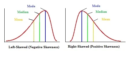
The value of skewness represents the extent, to which is the distribution curve distorted. If a set of data is symmetrically distributed, the value of the skewness is 0. In the case where the majority of data set values is concentrated on the left side, we talk about positive skewness. The average value of dataset is lower than the mean value. On the other hand, when the majority of data set values is concentrated on the right side, we talk about negative skewness. Now, the average value of the dataset is higher than the mean value.
Source: LaptrinhX
Why has the skewness of returns the power to predict the future returns?
There are two theoretical backgrounds that provide a possible explanation. Firstly and most importantly, the skewness preference literature argues, that the preferences of investors affect the demand for assets with particular distributional features (skewness). According to the theory, a specific type of investors have an intrinsic preference for positively skewed assets. This kind of investors searches for so-called lottery-like stocks, that could earn them a fortune, but with a very low probability. The demand for this kind of equities then leads to their overpricing and earning lower returns, than negatively skewed assets. Even if there is a possibility of short-selling, this overpricing is not fully arbitraged away. In the case of a positively skewed asset, the investors are not willing to open short positions, as they become exposed to the possibility of a significant loss. The second framework of skewness preference theories adds, that investors overweight the probability of occurring of the extreme events while underweight the occurring chance of events, that are most likely to happen.
Selective hedging represents the second mechanism, through which could skewness affect assets prices. It is a technique, in which the traders’ optimal hedge ratio is influenced by their expectations of future price movements. Therefore, their hedging positions turn more into speculation. If these type of hedgers have their preferences described by cumulative prospect theory or influenced by skewness, their goal would not be only to minimize the risk, but also maximize skewness.
Skewness across asset classes
Based on the idea of Skewness in Commodities, we have decided to follow in steps of an additional paper written by Nick Baltas and Gabriel Salinas: Cross-Asset Skew and test, whether the Skewness effect can be used to profit from also in other asset classes, and how can the presented strategy be further enhanced. So let’s check whether a similar trading strategy could also be applied for currencies, equities and bonds.
Skewness in currencies
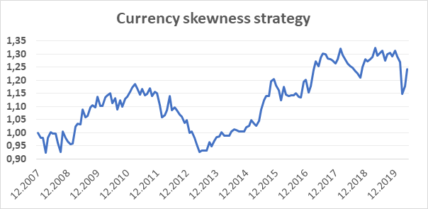
Our investment universe for testing the skewness effect in currencies consists of 8 CME futures contracts on the following currencies: AUD, GBP, CAD, EUR, JPY, MXN, NZD, CHF. Our dataset started in December 2006, and we have decided to follow the exact same strategy, as proposed in the first-mentioned paper (Fernandez-Perez at al.).
First of all, the skewness of returns has to be calculated for each trading day. In our test, we have calculated the skewness for day t based on the daily return of day t and daily returns of previous 259 trading days, which gives us approximately a yearly lookback period. Then we assess the skewness data of the last trading day in a month t-1, to create a portfolio in month t. Based on the assessment, we open a short position in two currencies futures with the highest skewness and long position in two currency futures with the lowest skewness on the first trading day of the month t. The portfolio is equally-weighted and held to the first trading day of month t+1 when its rebalanced according to the new skewness data. As the first skewness data are available at 12/31/2007, our trading sample starts from January 2008 and ends on May 2020. The presented strategy gained an annual return of 1,76%, with 8,87% yearly volatility, which gave us a 0,20 Sharpe ratio.
Skewness in equities
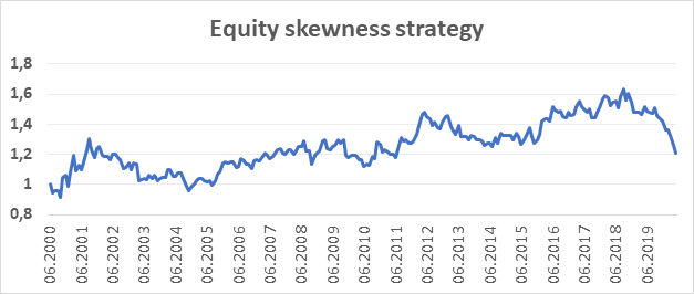
For equities, we have decided to test this effect with the same approach, as for currencies. Our equity investment universe is represented by futures contracts on eight different stock market indices: NASDAQ, DAX, S&P 500, SMI, EURO STOXX 50, CAC 40, FTSE 100 and Nikkei 225. Our data sample starts in June 1999, with the first skewness data available at 06/30/2000. Therefore, our trading sample starts in July 2000 and lasts until May 2020. Using the exact same strategy with going long on two instruments with the lowest skewness and short on two instruments with the highest skewness, the investor would achieve an annual return of 0,96% with equally-weighted portfolio. The annual yearly volatility reached 11,34%.
Skewness in fixed income
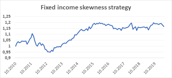
Finally, we have decided to test the same strategy also for fixed income assets. In our test, fixed-income assets are represented by seven different 10Y bonds futures. Our data sample begins in September 2009, meaning that first skewness data to be used are available at 10/29/2010. Our trading sample then begins in November 2010 and ends with May 2020. Since our universe consists only of 7 different instruments, the division into quartiles could not be followed exactly. Still, we decided to use the same principle: open long positions in the two bonds futures with the lowest skewness in returns and open short positions in the two bonds futures with the highest skewness. This time, the strategy would earn us an annual return of 1,62% with equally-weighted portfolio. With the annual yearly volatility at 4,78%, the strategy provides 0,34 Sharpe ratio.
Multi-asset skewness trading strategy
Skewness effect in all three other asset classes has positive results (albeit skewness in equities registered annoying drawdown in the last 12-months), but the resultant individual Sharpe ratios are far from satisfactory. But let us look deeper, how are the monthly returns of particular asset portfolios built on skewness effect correlated across asset classes.
| bonds | equities | currencies | commodities | |
| bonds | 1,00 | |||
| equities | 0,00 | 1,00 | ||
| currencies | 0,26 | 0,03 | 1,00 | |
| commodities | -0,06 | 0,08 | -0,14 | 1,00 |
The average correlation across our four asset classes portfolios was measured at just 0,03. Since there is almost no correlation between the monthly returns of the portfolios, it is reasonable to combine all four asset classes into one portfolio. Therefore, we can try to check a multi-asset strategy based on skewness effect, that would contain all four asset classes.
The compiled dataset that includes trading data for all four asset classes starts on November 2010 and ends in May 2020. One of the most crucial steps in our test was to assign the weights to the particular asset classes in our multi-asset portfolio. Since all of the assets shown different volatilities across different times, we have decided to follow the inverse volatility principle. For the first 12 trading months, the portfolio is equally-weighted across asset classes, since the volatility data are not available. Then, each asset class portfolio is assigned a weight inversely to its volatility in monthly returns in the past 12 months. The strategy with such a weighting achieved a 0,49 Sharpe ratio. However, the achieved annual return was only 1,99% with 4,06% yearly volatility.
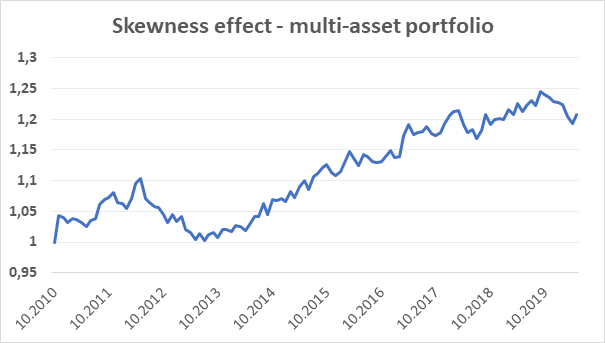
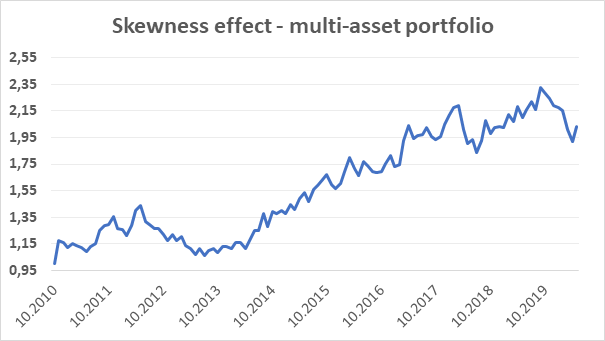
Since we use futures as our trading instruments, we can easily make a volatility target with leveraging our positions. In our sample, we have set our volatility target at 15%. For the first 12 trading months, where are no volatility data available, we have applied 1:4 leverage. We have used this value, as it later turned out to be approximately an average of used leverages across the whole sample period. After the first year, we leverage the position each month based on the past 12 month returns(not leveraged) volatility to reach our volatility target. So if the past 12-month volatility of un-levered strategy in month t-1 is measured at 5%, we use 1:3 leverage in month t. The strategy with using such a leveraging principle would earn 7,67% annual return from November 2010 to May 2020. With 15,57% yearly volatility, the Sharpe ratio has been measured at 0,49.
Conclusion
The best course of action for every quant researcher is to try fundamentally understand anomalies and explore their functioning besides the original scope of the academic research papers. The goal of this article was to look for inspiration and further explore the Skewness effect – the tendency of assets with the lowest skewness to outperform assets with the highest skewness. It seems that this anomaly is present not only in commodities but also in currencies, fixed income and equities. Trading strategy that exploits the effect of skewness in the multi-asset setting would earn an annual return of 7.67% when leveraged to the 15% volatility.
Authors:
Radovan Vojtko, CEO & Head of Research, Quantpedia
Marek Lievaj, Quant Analyst, Quantpedia
Are you looking for strategies applicable in bear markets? Check Quantpedia’s Bear Market Strategies
Are you looking for more strategies to read about? Sign up for our newsletter or visit our Blog or Screener.
Do you want to learn more about Quantpedia Premium service? Check how Quantpedia works, our mission and Premium pricing offer.
Do you want to learn more about Quantpedia Pro service? Check its description, watch videos, review reporting capabilities and visit our pricing offer.
Do you want algorithmic access to the full Quantpedia database via the API? Subscribe to Quantpedia Pro, ask for an API key, and explore the in/out-of-sample statistics, source academic papers, and code snippets — ideal for quantitative research, systematic trading workflows, and AI model training.
Are you looking for historical data or backtesting platforms? Check our list of Algo Trading Discounts.
Or follow us on:
Facebook Group, Facebook Page, Twitter, Linkedin, Medium or Youtube
Share onLinkedInTwitterFacebookRefer to a friend


