Pragmatic Asset Allocation Model for Semi-Active Investors
Introduction
The primary motivation behind our study stems from an observation of the Global Tactical Asset Allocation (GTAA) strategies throughout the existing papers – the majority of them require relatively frequent rebalancing from the point of view of the ordinary investor. Portfolio rebalancing is usually done on a weekly or monthly basis, and while this period may seem overly boring and slow for the majority of traders (who like to trade on intraday or daily basis), fans of GTAA strategies are not traders; they are investors. Of course, some like to follow the ebbs and flows of the market, read financial news, and like to be deeply involved in the process of building and testing strategies and picking just the right investments. But a lot of investors just want to have a life. The financial market is not their hobby. However, on the other hand, they also do not want to hold just the passive buy & hold portfolio (which they often see as too inert when something really important happens). Recognizing the demand for the semi-active strategy, we introduce our novel Pragmatic Asset Allocation.
We aim to reduce the frequency of rebalancing while retaining all the positive characteristics of GTAA strategies, such as global diversification, inclusion of multiple asset classes, and protection against downturns. We propose a quarterly rebalance with a minimum 12-month holding period, employing the common tranching approach (as used in our price-based country valuation article), where we only rebalance a specific pre-selected portion of the portfolio.
Moreover, in many countries, there are exceptions to taxes if you hold securities for more than 12 months. For example, in the United States, a long-term (instead of short-term) capital gains tax is applied to profits from selling an asset held for more than a year. The tax rate can be 0%, 15%, or 20%, depending on your taxable income and filing status. Generally, long-term capital gains tax rates are lower than short-term capital gains tax rates everywhere. And as it is said, there are only two certainties in life – death and taxes. So, to maximize this tax treatment, we devised innovative rules for GTAA strategies that maximized the optimization of taxes.
Related Literature
Global Tactical Asset Allocation (GTAA) is an investment strategy aiming to enhance returns and manage risk by dynamically shifting investments among various asset classes, such as stocks, bonds, and cash, depending on market conditions.
A crucial role in popularizing GTAA strategies played Meb Faber (2007), by writing one of the most popular papers that introduce the idea. The strategy was based on various moving averages/momentum filters to gain exposure to an asset class only when there is a higher probability for the outperformance of the simple buy-and-hold strategies but with much lower volatility and drawdowns. The paper’s results suggest that a market timing solution is a risk-reduction technique that signals when an investor should exit a risky asset class in favor of risk-free investments.
We have already examined how to Avoid Equity Bear Markets with a Market Timing Strategy, building trading signals based on price-based indicators, macroeconomic indicators, and a leading indicator, a yield curve, that can predict recessions and bear markets in stocks in advance. But this paper/strategy is only about the equity market, and one of the main features of the GTAA strategies is their multi-asset nature. Therefore, we had to broaden the scope of our model and include other assets.
We drew inspiration from the paper by Keller and Keunig (2016), who proposed a dual-momentum model using “crash protection” called Protective Asset Allocation (PAA). They moved all capital to cash or safe treasury bonds when global markets became more bearish. This approach integrates the research findings of Antonacci (2014), who extensively explored dual-momentum strategies by combining absolute momentum (trend following) and relative momentum (comparing momentum across assets).
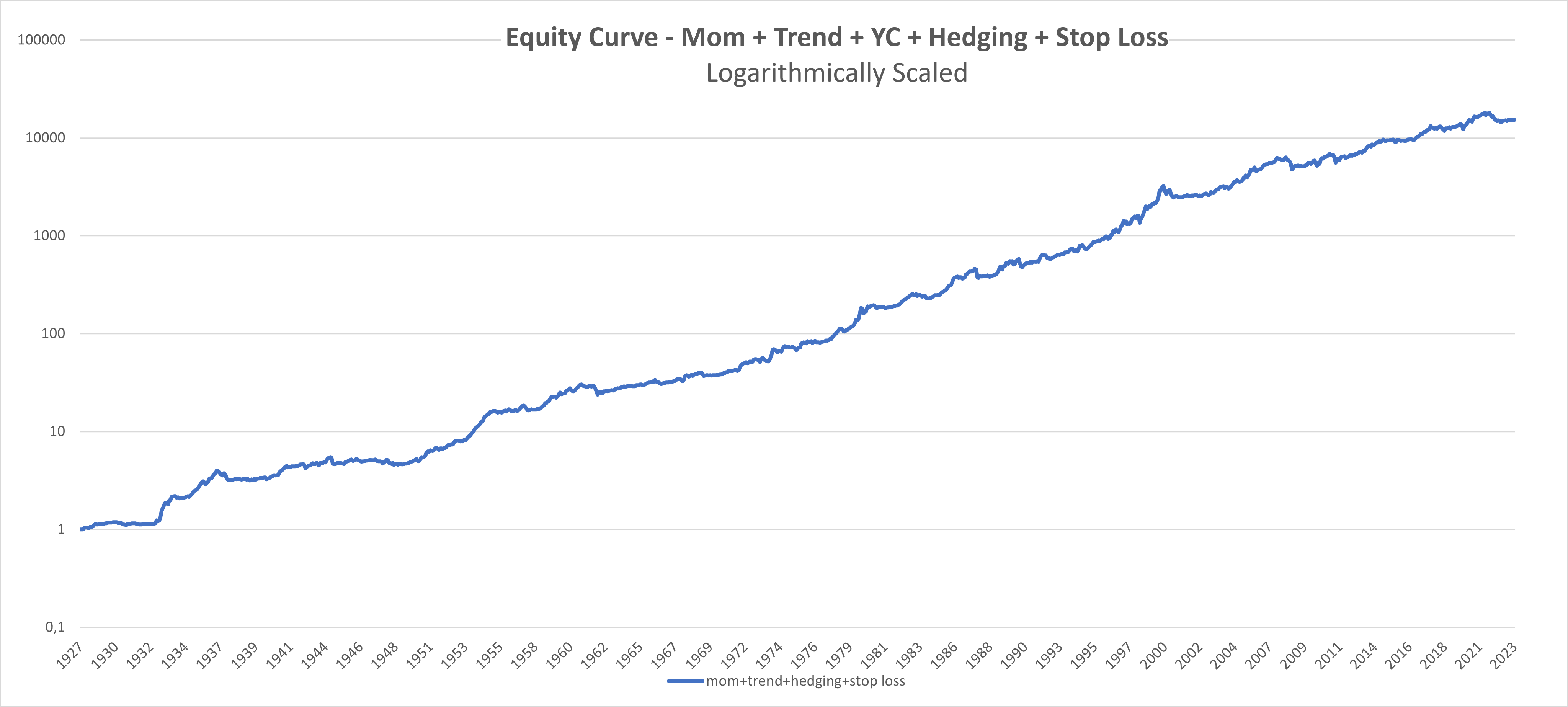
There are a lot of other studies that have explored the variations of the GTAA Strategy. But as we have already mentioned, most of the strategies on this theme that have already been published are rebalanced weekly or monthly. Therefore, we combined all main findings from our paper and the work of Maben Faber, Antonacci, and Keller&Keunig and brought a novel approach to the broad family of GTAA strategies by involving tranching and quarterly rebalancing while devising innovative rules to maximize the tax exceptions (a minimum holding period of 12 months for all assets in the portfolio). Moreover, we employed an extended time horizon starting in December 1927, allowing for a comprehensive historical perspective in our analysis. We also incorporated the Yield Curve preditor and replaced cash with a Hedging Portfolio. We used the Stop Loss mechanism to create one final trading strategy with an annual return of 10.73%, a Sharpe ratio of 0.93, and a maximum drawdown of only -23.98%.
Data and Methodology
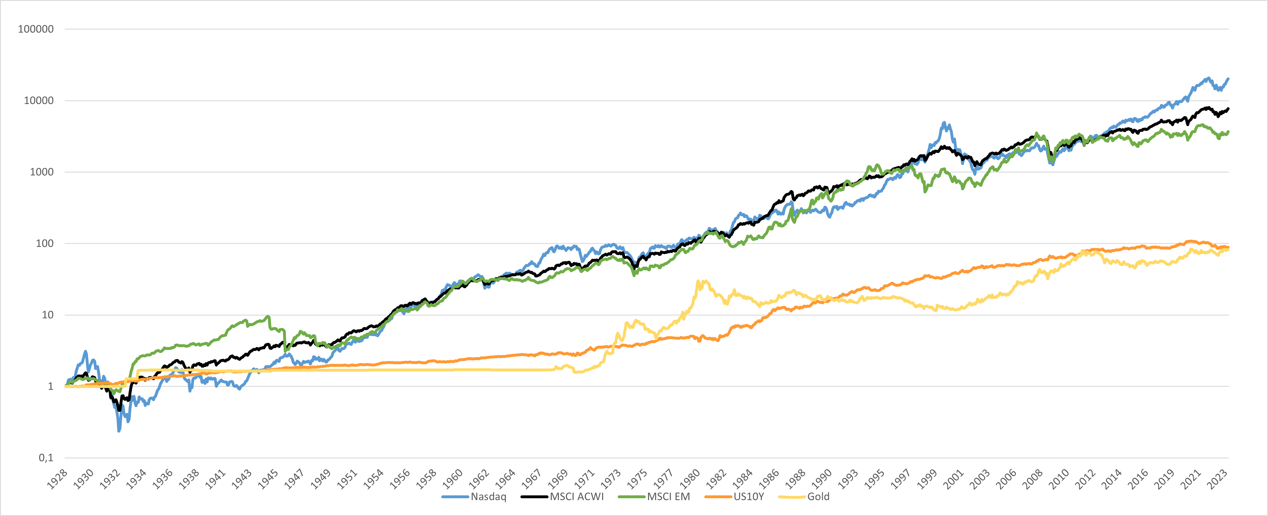
We backtested the models on the monthly data from December 1927 to August 2023. We use data from our database of global factors, from which we built the following set of assets (our investment universe):
- Nasdaq 100 Index: The Nasdaq Stock Exchange is known for listing many technology and internet-based companies and is considered to be one of the world’s largest and most well-known stock exchanges. We used the tech sector proxy before the index’s inception. The main reason we include this asset in our portfolio is to have exposure to the dynamic nature (with all of the ups and downs) of the innovations that stem from the tech stocks.
- MSCI ASWI (All Country World Index): The global equity index includes stocks from 23 developed and 27 emerging markets. It’s important to highlight that approximately 50% of the index is allocated to U.S. stocks, reflecting the significant weight of the U.S. It’s our main proxy for the equity risk, but it’s significantly less volatile and risky (and more diversified) than other two equity indexes we use.
- MSCI EM (Emerging Markets Index): The index tracking the performance of stocks from emerging market economies. These countries are considered to be in the early stages of industrialization with higher growth potential and risk than developed markets.
- US10Y: 10-year U.S. Treasury bonds can serve as hedge in times of global deflationary recessions.
- Gold: it is considered a hedge against inflation and a safe-haven asset during times of economic uncertainty.
Now we would like to spend some time explaining our rationale for the selection of our investment universe.
An observant reader may notice that our investment universe doesn’t include commodities, REITs, and a lot of other assets/ETFs (corporate bonds, EM bonds, etc.). It is not that the model would be worse with them – quite the opposite (we tried other variants). The reason is that we wanted to trim down the number of ETFs in our portfolio to a sufficient minimum due to ease of execution, but on the other hand, preserve the diversification of the portfolio. More assets would increase diversification, of course. But a lot of semi-active investors also do not like to juggle a lot of different ETFs/categories. Therefore, we omitted a lot of possible additions from our model and stuck to just 3 “risky” assets (tech, world, em stocks) and 2+1 safe assets (us treasuries, gold, and cash). Additionally, having fewer assets simplifies the job of obtaining sufficient history for all of the assets. Building an EM stocks proxy was a hard job in itself (we may write an article about that in the future).
One last thing needs explanation. Why did we pick the EM, tech, and global equities as the main risky assets? We will try to explain our reasoning here.
The model from which we started to build our Pragmatic Asset Allocation is our paper Avoid Equity Bear Markets with a Market Timing Strategy, but this paper uses only the US equities as the investment universe. We wanted to retain the usage of equities as the primary driver of the performance. We acknowledge other risky assets offer risk premiums – like commodities, REITs, corporate bonds, crypto, infrastructure, collectibles, etc. However, we consider equities to be the primary risky asset that has a lot of advantages (liquidity, ease of access) and offers sufficient risk premium. Other assets have short-comings in some of the characteristics, be it liquidity (infrastructure, collectibles, REITs), questionable size of the risk premium (commodities), hybrid assets (corporate bonds and REITs are usually just a mixture of equity and duration risk, and do not add a lot from the diversification perspective) or do not have sufficient history (crypto, alternatives).
Of course, we wanted to expand from the US equities to the world index, and the All-Country Index seems to be the best proxy. But then, we wanted to have the ability to tilt our risky portfolio. Equities are sensitive to the business cycle, and individual segments of the stock market react differently. Investors can increase or decrease exposure to individual sectors (energy, health care, tech), countries, or whole regions (US, EU, EM, Asia, etc.). There is not just one way how to do it and which sectors/countries/regions pick for the tactical part of the model. In the end, we decided to pick the EM region (based on our analysis of the cyclicality of the outperformance of the US market against the EM region) and tech stocks segment (we wanted to have a high-beta segment of equities for strong uptrends in equities, that is not correlated to EM region performance and tech stocks fulfill this perfectly).
We do not imply, that this is the best selection of risky assets, but it suits our needs the best. Of course, you – our readers, are welcome to try different investment universes on your own.
And at the end, a few last words about the selection of the “hedging” or “safe” assets, which are 10Y US Treasuries, Gold, and cash, in our case. We wanted to have an asset that works well in deflationary recessions (10Y Treasuries), one for inflationary periods (Gold/Commodities), and one asset that works well when there is a recession caused by a lack of trust in public institutions (Gold/cash). In the end, we gravitated towards the classical trio, and we will let the price/model tell us which asset is the best store of value for each period.
Holding Periods and Execution Techniques
As mentioned in the Introduction above, we decided to reduce the frequency of rebalancing while preserving all the positive characteristics of GTAA strategies, and even more – we devised innovative rules for GTAA strategies to optimize taxes. In many countries (and also ours), there are exceptions to taxes if you hold securities for more than 12 months. The best way to maximize tax exceptions while quarterly rebalancing is tranching. There are different approaches to tranches with varying holding periods and rebalancing frequencies, for example:
- 4x tranche, 12-month holding period (1 year), quarterly rebalancing,
- 12x tranche, 36-month holding period (3 years), quarterly rebalancing,
- 10x tranche, 60-month holding period (5 years), half-year rebalancing.
Source: Tranches (wallstreetmojo.com/tranches)
We decided on the first option: to divide the portfolio into four sub-portfolios; each part is rebalanced once per 1 year and is weighted as 1/4 of the weight in the full portfolio. Quarterly rebalancing is, for example, done 31.1, 30.4, 31.7, and 31.10 each year.
So explained:
31.12.1927, we calculate the signal for the first individual tranche, apply one month waiting period (we will discuss that later), and invest accordingly at 31.1.1928, which we hold until 31.1.1929 when we rebalance again for a 1-year holding period. Similarly, in 31.3.1928, we calculate the signal for the second individual tranche, then 30.4.1928 is being invested the second 25%, which we hold until 30.4.1929. The same is done for 31.7.1928, held until 31.7.1929, and finally, 31.10.1928, held until 31.10.1929. The final portfolio is equally weighted among four tranches; each tranche is rebalanced once a year.
Why do we apply a 1-month pause between signal generation and actual rebalancing? Because we want to be realistic. Of course, the model gives slightly better results when tranches are rebalanced right after the signal is generated – so at the close of the last trading day of the quarter or the soonest afterward, which is usually the next trading day. But remember, we are trying to build a model for semi-active investors. So, by postponing the actual portfolio rebalancing from the signal generation by one month, we give semi-active investors enough time to perform the needed portfolio adjustments.
The Pragmatic Asset Allocation model isn’t very sensitive to actual date of the rebalancing. Of course, there is some luck involved, and some days of the month can be better than others. But it’s firstly an investment model framework, not a swing trading strategy. It tries to capture longer-term moves in prices of the underlying assets, not intra-month variations. It also deliberately leaves some gap between the time of the signal and the portfolio rebalancing date for those who like to catch intra-month lows. Can you execute the signal better than at the end of the next month because you believe you have a good market entry strategy? Then just go for it! You may add some alpha; we’re keeping our fingers crossed for you.
Portfolio Construction
Starting with the investment portfolio of Nasdaq, MSCI ASWI, and MSCI EM, we systematically created the strategy in six progressive steps, with each stage adding unique elements to enhance the overall portfolio:
- Momentum
- Trend
- Cash
- Yield Curve
- Hedging Portfolio
- Stop Loss
Let’s delve into the details of each step of your strategy construction:
1. Momentum
Momentum, one of the most well-known strategies, refers to the persistent tendency of assets to continue their recent trends. The core concept behind momentum investing is the belief that assets that have performed strongly over a specific time frame will likely sustain that positive performance. Conversely, assets with a history of poor performance will continue in that negative direction.
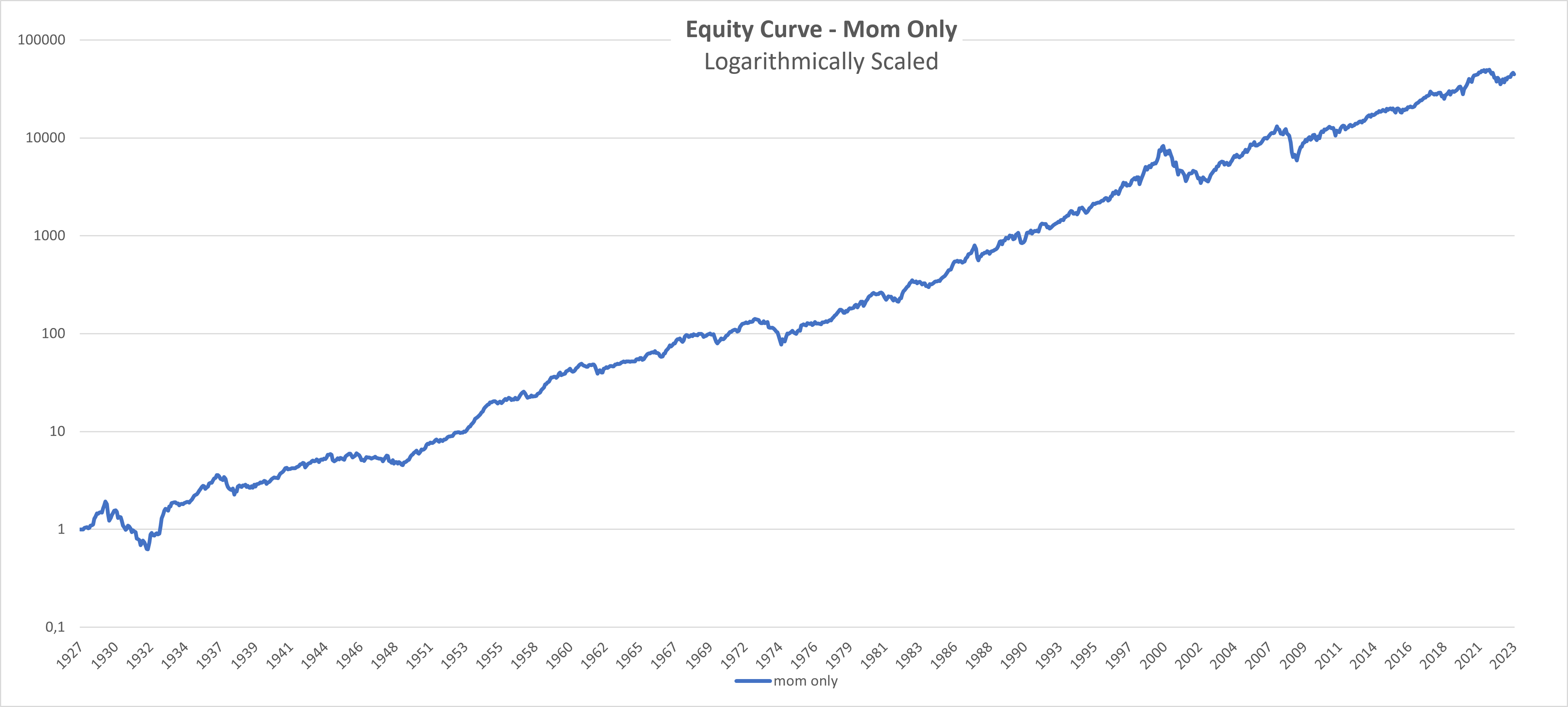
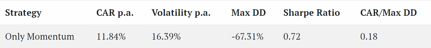
Our initial strategy integrates three assets: Nasdaq, MSCI ACWI, and MSCI EM, employing only momentum. We select the top two (out of three) assets based on their 12-month momentum (monthly performance/monthly performance before 12 months – 1).
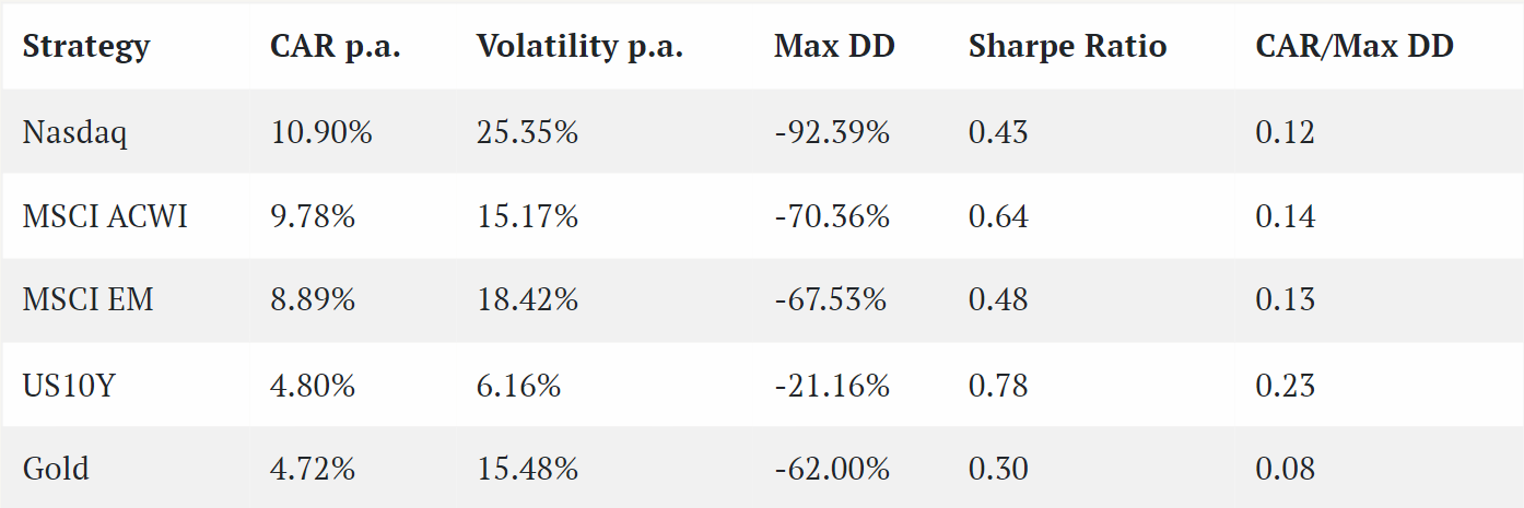
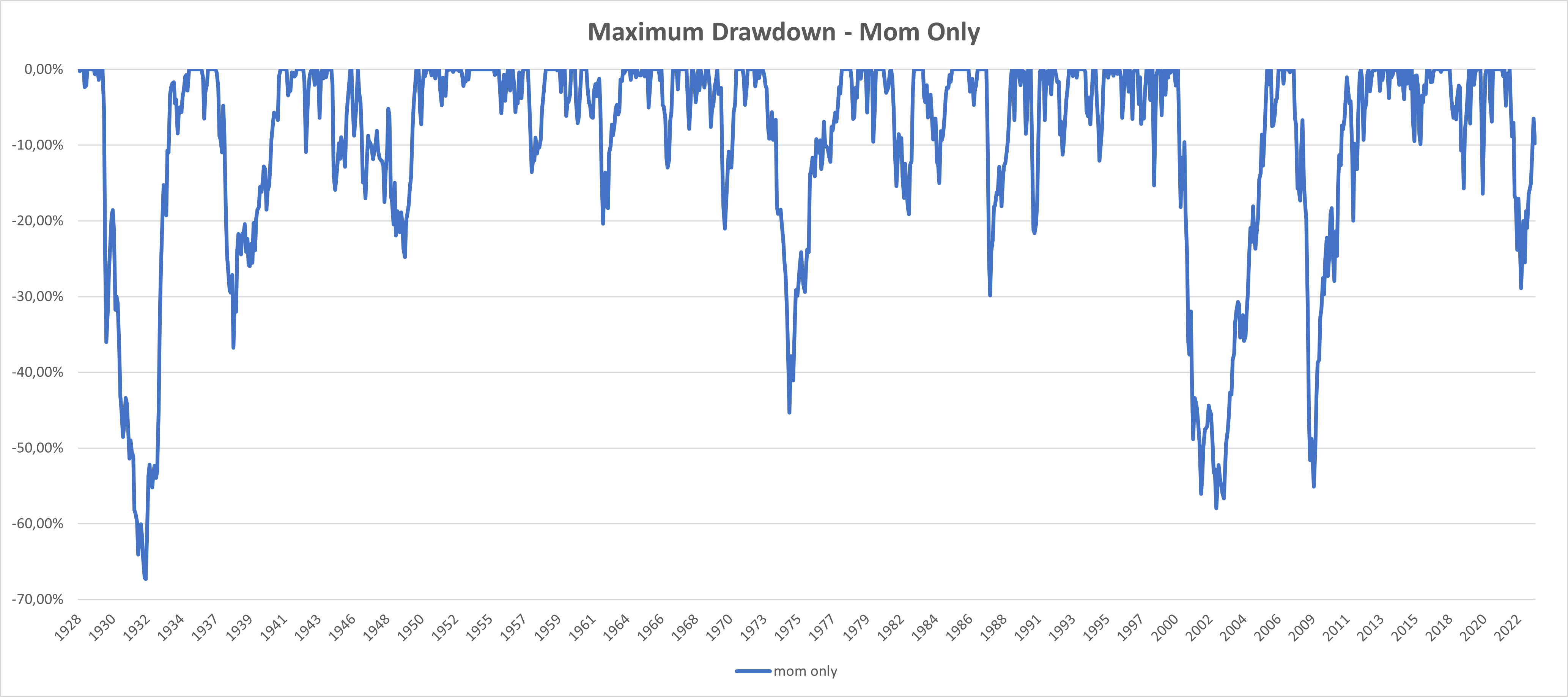
The strategy exhibits a CAR (Compound Annual Return) of 11,84%, indicating improvement compared to all three assets (Nasdaq – 10.90%, MSCI ACWI – 9.78%, MSCI EM – 8.89%). We have better performance because we rotate to high-beta segments (EM, Tech) when the price signals us to do so. However, it’s crucial to acknowledge the relatively high maximum drawdown (-67.31%). Strategy is always invested in the equity market; we just change the portfolio’s composition (sectors/regions). So, there is no way to avoid large drawdowns. In all of the following steps, we will optimize the portfolio by actively seeking to decrease the maximum drawdown while preserving the momentum’s alpha against the simple buy-and-hold strategy.
Do not forget that the investment strategy rebalances quarterly and always only 25% of the portfolio. So, into the first tranche, we can select 2 assets, each with the 12.5% weight, then 2 assets into the 2nd tranche, each with 12.5% weight, 3 months later, etc., etc.
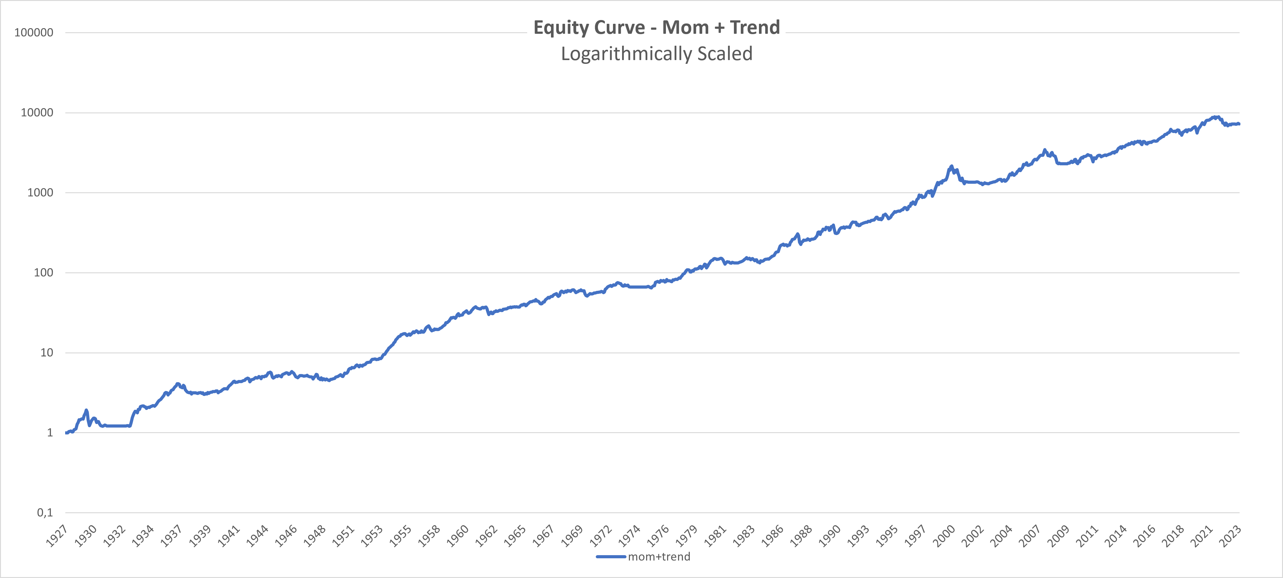
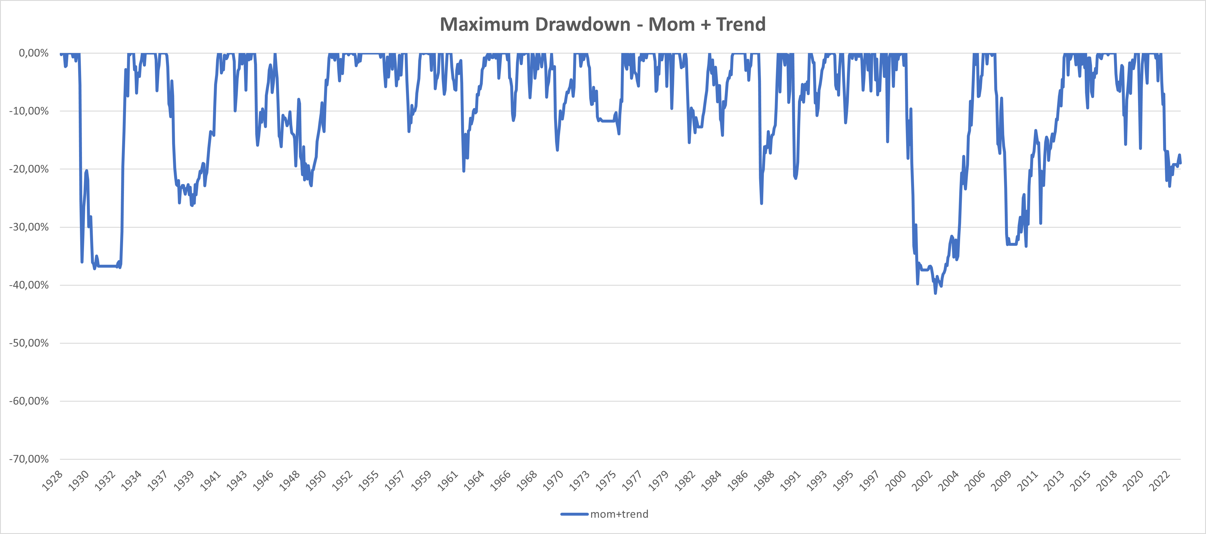
2. Trend
In the second step, we introduced the trend component to the momentum strategy, drawing inspiration from the dual momentum strategy by Meb Faber (2007), or Antonacci (2014). Firstly, we calculated the 12M moving average. We are in an uptrend if monthly performance is higher than the average of the last 12 months. Otherwise, we are in a downtrend. To reduce the risk, we choose an asset only if it is in an uptrend.
In summary of our first and second steps, we select two of the three assets based on their performance, giving 12.5% weight to each asset, but only if they are not in a downtrend. If one asset (out of the 2 we picked) is in a downtrend, then it is omitted from the portfolio for the next 12 months, and the remaining asset gets 12.5% weight. If both assets are in a downtrend, we are not invested in that particular tranche in anything for 12 months. While the trend-following strategies are recognized in various papers, our strategy’s unique value proposition stems from the implementation of tranching and quarterly rebalancing approach.
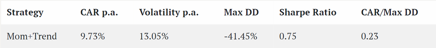
We have effectively mitigated the maximum drawdown compared to the first step, reducing it significantly from -67.31% to -41.45%. It’s important to note that this improvement in maximum drawdown comes with a trade-off, as the return has decreased from 11.84% to 9.73%. It’s a significant hit to the performance, but we can repair it.
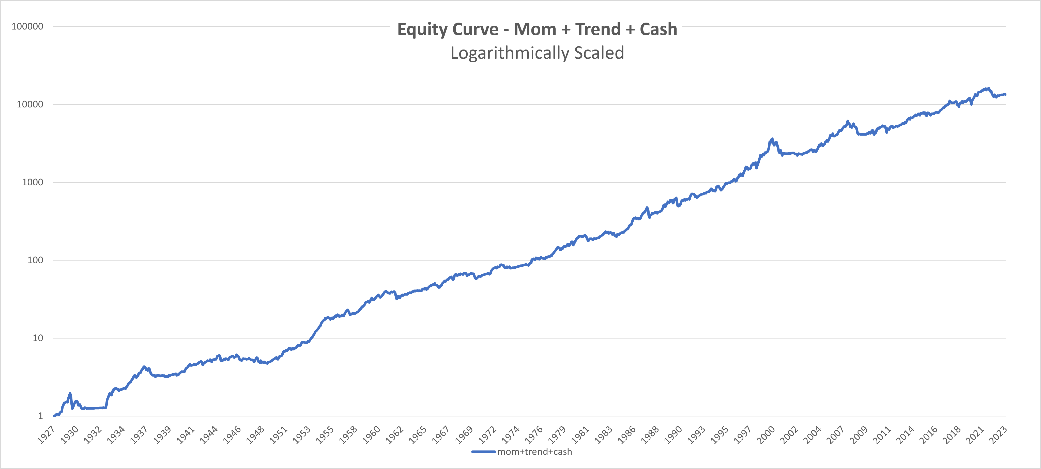
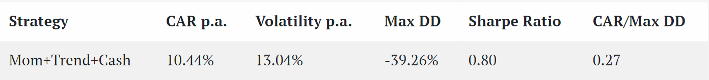
3. Cash
In the next step, we incorporated a cash component into the strategy to enhance the returns by strategically allocating to cash when our model signals a lack of riskier assets. For example, when two of our three assets are in a downtrend, we choose only one that is in uptrend and allocate 12.5% in cash. On the other hand, when all three assets are in a downtrend, we invest 25% (the whole tranche) in cash .
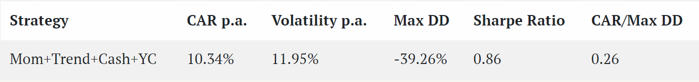
This approach increased returns (from 9.73% to 10.44% compared to the previous step) and reduced the maximum drawdown (from -41.45% to -39.26% compared to the previous step). By integrating cash into our strategy, we optimized the portfolio’s performance, achieving a higher return on investment while minimizing the potential losses. Better, but there are still some things we can do.

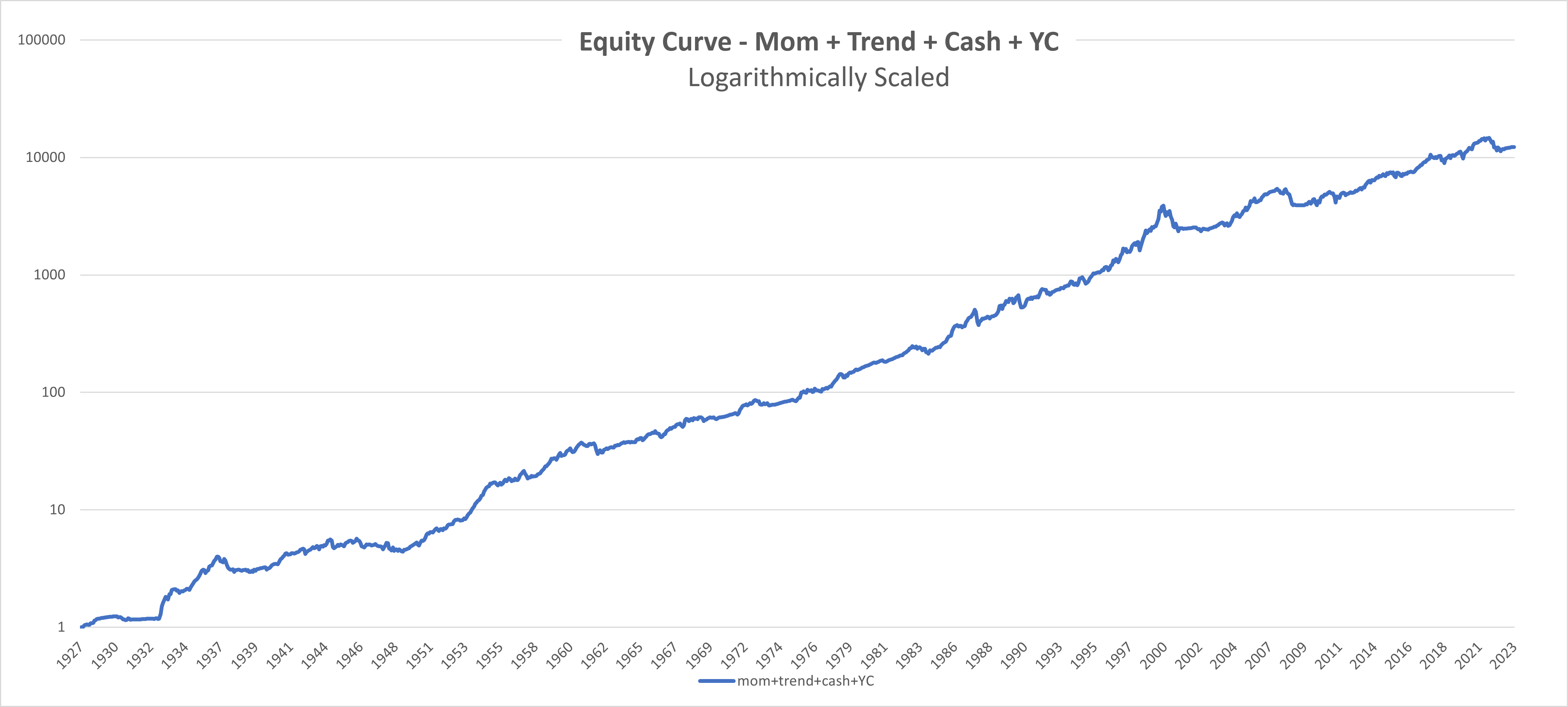
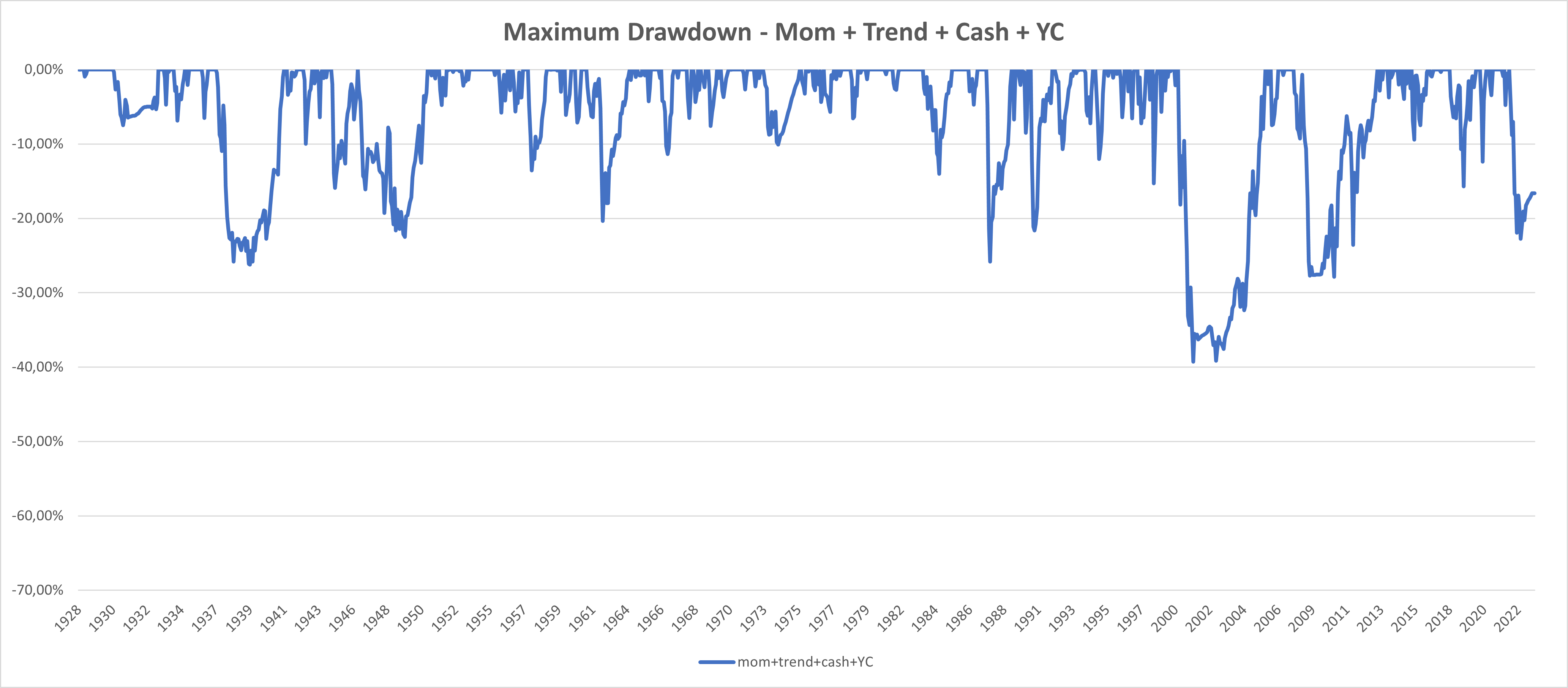
4. Yield Curve
The Yield Curve (YC) is a valuable indicator of the connection between short and long-term interest rates for fixed-income securities issued by the U.S. Treasury. Normally, the yield curve exhibits an upward slope, reflecting that long-maturity debt is associated with higher rates than shorter-term obligations. However, the yield curve inverts when short-term interest rates exceed long-term rates. An inverted yield curve is uncommon because it indicates that the near-term is riskier than the long-term.
The monetary policy and investor expectations influence the yield curve’s slope. Rising short-term rates due to the implementation of expansionary monetary policy could slow economic activity and demand as borrowing becomes more expensive. Simultaneously, slowing activity may result in lower inflation, increasing the probability of a future monetary policy easing. This expectation of future rate cuts can lead to an inversion of the yield curve as investors anticipate lower interest rates, which explains the relationship between the yield curve and recessions.
In this part, we have utilized the approach from our article Avoid Equity Bear Markets with a Market Timing Strategy – Part 3. Firstly, we calculated the YC Signal. The YC Signal tells us to stop investing in our investment universe (stay only in Cash) when the 3-month U.S. Treasury yield exceeds the 10-year U.S. Treasury yield. In this step, we also explored the integration of macro factors (the idea comes from our previous article – Avoid Equity Bear Markets with a Market Timing Strategy – Part 2). However, due to the quarterly rebalancing and tranching methods employed, the impact of macro factors was limited, leading us to decide against their inclusion in our strategy. Integration of the macro factors would improve strategy, but just by a very little. So, we decided not to overcomplicate the strategy with an additional layer of macro-signals.
Incorporating the yield curve into our strategy adds significant value by effectively reducing portfolio volatility from 13.04% to 11.95%. Consequently, as a direct result, the Sharpe ratio, a key metric for risk-adjusted returns, has improved, rising from 0.8 to 0.86.
5. Hedging Portfolio
Gold and US10Y are often preferred components for a hedging portfolio due to their distinct characteristics in times of market uncertainty. Gold is in general considered a hedge against inflation and a safe-haven asset during economic uncertainty. At the other time, investors seek the safety of government bonds, particularly those issued by economically stable countries like the United States. The two assets have a low correlation with each other and traditional equity markets, enhancing the portfolio’s overall diversification.
Firstly, we “duplicated” the first two steps (Momentum+Trend) utilizing Gold, US10Y, and Cash. We selected two of the three assets based on their performance, but only if they are not in a downtrend, creating our hedging portfolio.
Secondly, we replaced the Cash in step 4. with our Hedging Portfolio. When YC Signal tells us to invest, and two of our three assets (Nasdaq, MSCI ACWI, MSCI EM) are in a downtrend, we choose only one and allocate 12.5% to Hedging Portfolio. On the other hand, when all three assets are in a downtrend or when the YC Signal tells us to stop investing, we allocate 25% in the Hedging Portfolio.
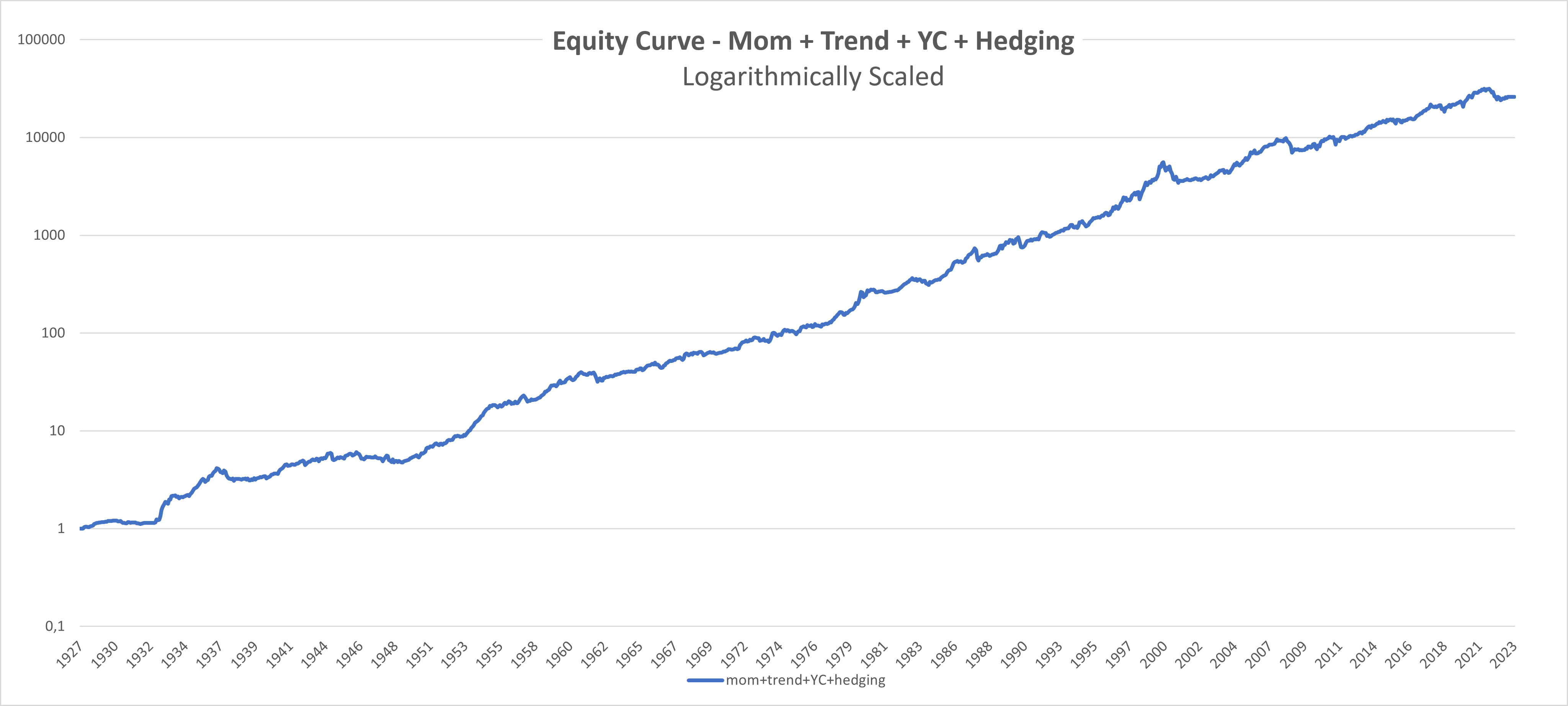
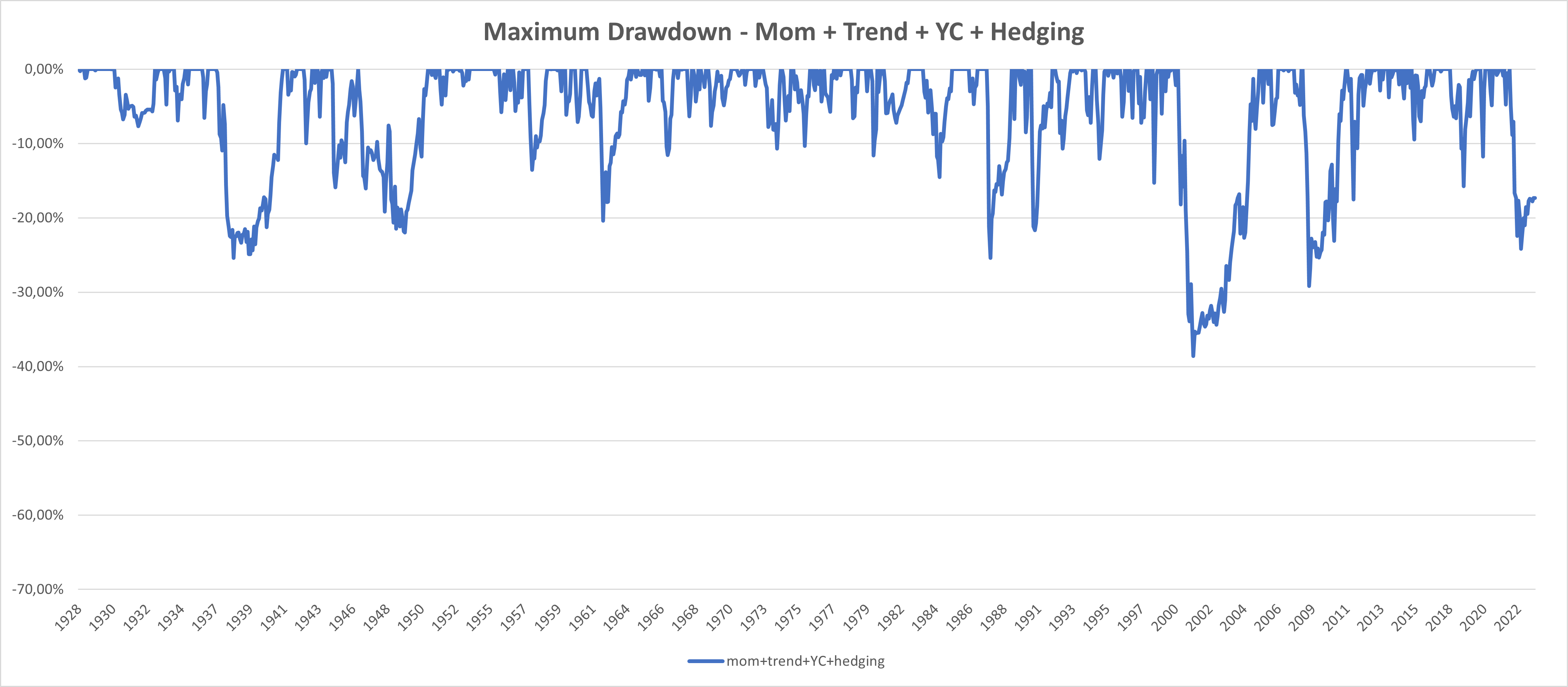
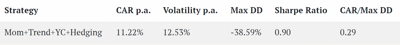
Utilizing the Hedging Portfolio helped us to increase the return in comparison to the previous step (from 10.34% to 11.22%) at the same time enhancing the Sharpe Ratio (from 0.86 to 0.90) and improving the Sortino Ratio (CAR/Max DD) from 0.26 to 0.29.
That’s a nice improvement, but is there still one more step that we can take to improve the whole strategy? Do any one of you, our readers, have any guess?
6. Stop Loss
In our final step, we decided to reduce the maximum drawdown of our strategy, implementing the “Stop Loss” mechanism. Let’s show an example of how the “Stop Loss” works:
On March 31, 2007, the strategy selected MSCI World equities, and we held them for one year, from April 30, 2007, until April 30, 2008, when the signal indicated that we could continue holding them. However, since the 12-month period has already passed, we could sell the ETF before April 30, 2009, as there would be no tax implications, having already reached the long-term capital gains tax period. If the moving average signal changes sooner, for example, on June 30, 2008, we can comfortably sell later, on the next tranche rebalancing day (on July 31, 2008), without waiting until April 30, 2009, when we normally should rebalance this particular tranche.
The stop-loss check is done only on usual quarterly dates (December 31, March 31, June 30, September 30). So when the stop-loss is activated, the investor does not trade outside of the usual quarterly time frame; he just sells the position that hits “stop loss” next month, when the other tranche may be rebalanced, too.
Of course, if you, the readers, want the model to be amended to react faster, check stop-loss on a monthly basis, and sell right away, the results would be even better. But once again, we opted for being conservative, and our implementation waits for the quarterly stop-loss check and position liquidation.
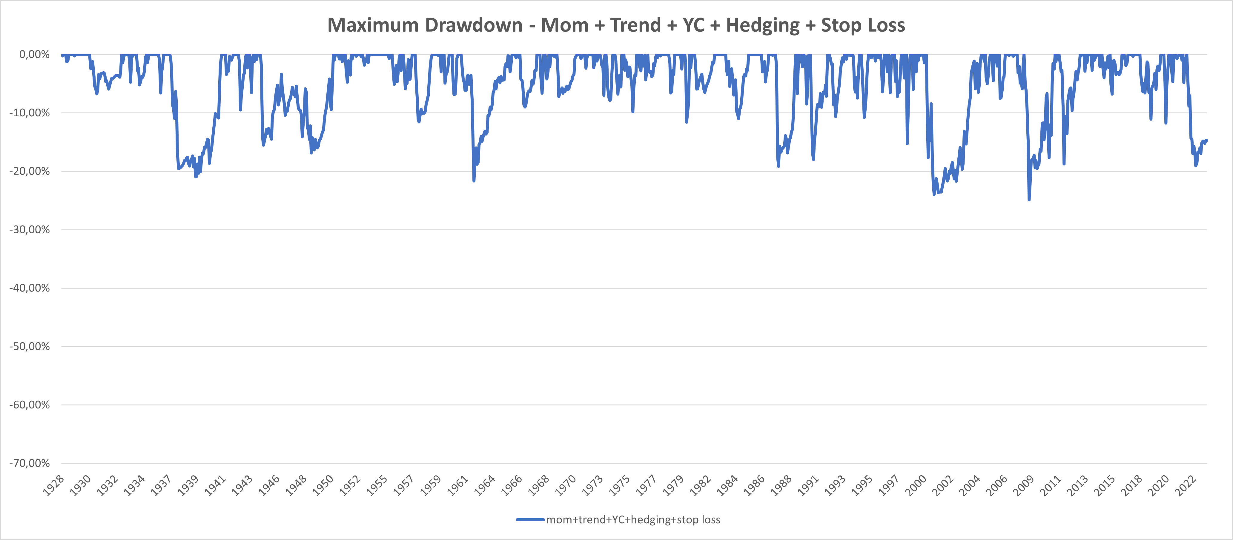
The “Stop Loss” significantly reduced the maximum drawdown (from approximately -38% to around -24% compared to the previous step), making it our final version. A maximum drawdown of around -24% is likely the best we can expect from a strategy of this kind. For example, in 1987, equity indices dropped around -20% in a single day, so our -24% drawdown on monthly data with quarterly rebalancing in such a mildly active strategy is at the limit of what can be achieved.
Is -25% to -30% too much for you? Then, the only possibility is to combine this semi-active model with a passive portfolio of low-risk securities (short- to mid-term bonds and/or cash). Or you must use models that are significantly more active.
| Strategy | CAR p.a. | Volatility p.a. | Max DD | Sharpe Ratio | CAR/Max DD |
|---|---|---|---|---|---|
| Mom+Trend+YC+Hedg+SL | 10.73% | 11.48% | -23.98% | 0.93 | 0.45 |
Conclusion
Our GTAA strategy represents an innovative investment approach, introducing unique mechanisms to optimize returns and manage risk while preserving the positive characteristics of GTAA strategies, such as global diversification, inclusion of multiple asset classes, and protection against downturns. We have integrated Momentum, Trend, Cash, Yield Curve, Hedging Portfolio, and Stop-Loss mechanisms into our strategy through a six-step process. Adding other assets like commodities, cryptocurrencies, or real estate investment trusts (REITs) to the portfolio was considered, but we decided not to overcomplicate things in this article.
Incorporating tranching, quarterly rebalancing, and a focus on tax optimization distinguishes our strategy from existing GTAA approaches. While incorporating tax optimization into investment strategies is logical, implementing innovative rules for Global Tactical Asset Allocation GTAA strategies that truly optimize taxes is relatively rare. Tax optimization can significantly enhance investment portfolios’ overall performance and efficiency.
The extensive historical analysis from December 1927 to August 2023 provides a thorough perspective on the strategy’s performance across various market conditions. The final version of our GTAA strategy demonstrates a balanced trade-off between risk and return, with an annual return of 10.73%, a Sharpe ratio of 0.93, and a significantly reduced maximum drawdown.
Share onLinkedInTwitterFacebookRefer to a friend


