Introduction

The Efficient Market Hypothesis (EMH), theory developed in the 1960s, states that stock prices reflect all available information, making it impossible to consistently earn above-average returns using this information. Nevertheless, numerous studies challenge this view by documenting anomalies that suggest markets may not be fully efficient. One group of such anomalies, known as calendar anomalies, demonstrate predictable patterns in stock returns linked to specific times.

Video summary:

Motivation

In one of our older posts titled ‘Case Study: Quantpedia’s Composite Seasonal / Calendar Strategy,'[11] we offer insights into seasonal trading strategies such as the Turn of the Month, FOMC Meeting Effect, and Option-Expiration Week Effect. These strategies, freely available in our database, are not only examined one by one, but are also combined and explored as a cohesive composite strategy. In partnership with Deltaray, using MesoSim — an options strategy simulator known for its unique flexibility and performance[5] — we decided to explore and quantify how our Seasonal Strategy performs when applied to options trading. Our motivation is to investigate whether this strategy can be improved in terms of risk and return. We aim to systematically harvest the VRP (volatility risk premium) timing the entries using calendar strategy to avoid historically negative trading days.

In the following sections, we will briefly discuss academic studies in the area of calendar anomalies, we then describe the data preparation process and the four steps involved in developing our final strategy.

Relationship to Literature

As early as 1962, Osborne observed an interesting weekly pattern: U.S. stock markets experience significantly lower returns on Mondays and higher returns on Fridays compared to other weekdays[6]. Investors have been keen on exploiting similar temporal anomalies ever since. Building on this, the January Effect, documented by Rozeff and Kinney in 1976, shows that returns in January are unusually high compared to other months[7]. Further expanding on monthly trends, Ariel highlighted the Turn-of-the-Month Effect, where the end of one month and the start of the next typically see higher returns, suggesting an optimal strategy of buying SPY ETFs at month’s end and selling at the beginning of the next[2]. The Payday Effect, similar to the Turn of the Month, is triggered around typical payday schedules, particularly on the 15th and at month-end, when employees often invest their paychecks[4]. This offers another profitable opportunity to buy SPY ETFs on these days and sell them shortly after. Additionally, the market exhibits predictable patterns around specific events such as Federal Open Market Committee (FOMC) meetings, where the S&P 500 generally performs better, possibly in reaction to the Federal Reserve’s decisions aimed at stabilizing and enhancing the economy[9]. By purchasing SPY ETFs the day before an FOMC meeting and selling them afterward, investors can capitalize on the market’s typically positive response. Another trading window is the Option-Expiration Week Effect, observed during the week leading up to the regular expiration of options—the Friday before the third Saturday of each month. During this period, stocks with large market capitalizations and active options trading tend to yield higher returns[8].

These patterns are just a few examples of the many calendar effects observed globally, which range from those related to the Islamic calendar[1] to events like the FIFA World Cup[3]. Each highlights potential inefficiencies in market behavior. Such effects significantly shape our modern trading strategies. Through our collaboration with Deltaray, we explore these anomalies to develop strategies that could lead to better risk-adjusted returns with focus on options trading.

Data Preparation

First, we created a Google Sheet for our data, where each row represents a date.

Column A includes dates within the backtest time range, each marked with a 9:30 AM timestamp. This timing ensures that MesoSim can use the data on the same day.

Column B tracks when regular options expire. We use a formula that checks if the date in Column A is the third Friday of the month. Third Friday of the month is when these options typically expire. If there is a match, the date is marked with a ‘1’. Formula runs as follows:

=if(date(Year(A2), month(A2), day(A2)) = (DATE(YEAR(A2),MONTH(A2),1+7*3)-
WEEKDAY(DATE(YEAR(A2),MONTH(A2),8-6))), 1, 0)

This formula calculates if the given date aligns with the third Friday by subtracting the weekday number of the second day of the month from the 22^nd.

Column C, the ‘option expiration week’, calculates and marks the whole week leading up to each expiration date using the formula:

=if(countif(B2:B6, “=1”) > 0, 1, 0)

If there is a cell in a given range that contains ‘1’, it means that the week includes an option expiration day. Any week containing an expiration date is marked with a ‘1’.

Column D, the ‘option expiration week start’, signals when the expiration week starts. This happens when the marks in Column C change from  ‘0’ (no expiration week) to ‘1’ (start of expiration week) between two rows. This column will be used by MesoSim to trigger trades Formula:

=if(and(C2 <> C1, C2 = 1), 1, 0)

To see when one month changes to the next, we create a Column E ‘end of the month’ using the formula:

=if(month(A2) <> month(A3), 1, 0)

This checks if the month of the current row is different from the next and marks the transition with a ‘1’.

Given that the end-of-month period is already covered by the Turn of the month represented by Column E, we also marked the mid-month payday, happening around the 15^th in Column G:

=if(day(A2) = 15, 1, 0)

Column F includes the dates of the FOMC (Federal Open Market Committee) meetings. These dates can be sourced from financial calendars like Investing.com[10].

Our fully prepared Sheet can be accessed here: https://docs.google.com/spreadsheets/d/1hUo-De3z2QqLV5iL-X90a60sO0vXlCAY626ETTsZUOU/edit?usp=sharing

Approach

The analysis consists of four steps: setting up synthetic long positions using options, applying a volatility risk premium (VRP) strategy, incorporating stop-loss mechanisms to manage risks, and optimizing position sizing for better risk management. Each step will be described in detail.

Step 1: Synthetic Long using Options

In our original paper and backtest we use SPY ETF. As MesoSim is an option-only backtester, they use a synthetic long position on SPX to match the SPY-based investment strategy. Synthetic Long consists of simultaneously Buying a Call Option ATM and Selling a Put Option ATM. These two actions mimic buying the SPY ETF and represent a simple way to replicate our strategy using options.

Backtest results can be viewed here: 
https://mesosim.deltaray.io/backtests/769b2a40-03b4-4ef3-b397-353f50ee0c01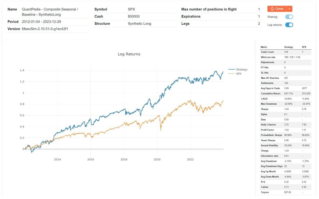

QuantPedia Composite SyntheticLong Overview

Expiration selection

We use options expiring nearest to 5 DTE in case of option_expiration_week_start and end_of_month signals. For any other signal (fomc, payday) we pick 1 DTE options.

Respective configuration section:

“Expirations”: [
     { 
    “Name”: “exp1”,
    “DTE”: “(option_expiration_week_start == 1 or end_of_month == 1) and 5 or 1”,
    “Min”: “1”,
    “Max”: “5”,
     }
     ]

Structure / Leg definitions

We use the Statement Selector to pick strikes using the underlying price as target for the short_put leg. The long_call leg will use the same strike as the short put leg, using the leg_short_put_strike variable.

Respective configuration section:

“Legs”: [
     {
           “Name”: “short_put”,
           “Qty”: “-1”,
           “ExpirationName”: “exp1”,
           “StrikeSelector”: {
           “Statement”: “underlying_price”
           },
           “OptionType”: “Put”
     },
     {
           “Name”: “long_call”,
           “Qty”: “1”,
           “ExpirationName”: “exp1”,
                “StrikeSelector”: {
                “Statement”: “leg_short_put_strike”
           },
           “OptionType”: “Call”
     }

Entry definition

We will enter whenever the signals defined in the Google Sheet is set to 1. We use the column-names defined in sheets as variables:

fomc_today, end_of_month, option_expiration_week_start, payday

We allow one Position in flight and we try to enter every day, 5 minutes after open:

“Entry”: {
     “Schedule”: {
     “AfterMarketOpenMinutes”: “5”,
     “BeforeMarketCloseMinutes”: null,
     “Every”: “day”
     },
     “Conditions”: [
           “fomc_today == 1”,
           “end_of_month == 1”,
           “option_expiration_week_start == 1”,
           “payday == 1”
     ],
     “VarDefines”: {},
     “AbortConditions”: [],
     “ReentryDays”: “1”,
     “Concurrency”: {
           “MaxPositionsInFlight”: “1”,
           “EntryShiftDays”: “1”
     },
     “QtyMultiplier”: null
  },

 Exit definition

We exit the trade on the last trading day. Alternatively, we could run it into settlement.

“Exit”: {
     “Schedule”: {
     “AfterMarketOpenMinutes”: null,
     “BeforeMarketCloseMinutes”: “5”,
     “Every”: “day”
     },
     “MaxDaysInTrade”: “expiration_exp1_dte”,
     “ProfitTarget”: null,
     “StopLoss”: null,
     “Conditions”: [],
     “VarDefines”: {}
  }

External Data and Simulator settings

We leverage MesoSim’s External Data capabilities to load the data prepared in Google Sheet and use it as signal for entry. To have a realistic simulation we set the Commission to $1.5 / contract and set the fill model to Mid Price. Slippage is disabled for this experiment:

 “ExternalData”: {
     “CsvUrl”: “https://docs.google.com/spreadsheets/d/e/2PACX-1vRei87mgnKNW-1dehmQwYzipn47J8cyhPRsZom50J_jH5OY1jY23aOeD9sglzLph9sRUgf8qVbWAm3f/pub?output=csv”
  },
  “SimSettings”: {
     “FillModel”: “AtMidPrice”,
     “SlippageAmt”: “0”,
     “Commission”: {
     “CommissionModel”: “FixedFee”,
     “OptionFee”: “1.5”,
     “DeribitCommissionSettings”: null
     },
     “LegSelectionConstraint”: “None”,
     “Margin”: {
     “Model”: “None”,
     “HouseMultiplier”: null,
     “RegTMode”: “CBOEPermissive”
     }
  }

As for results, when comparing the run with S&P Buy and hold performance we notice that the time in trade is reduced to 1/3rd and Sharpe is increased from 0.78 to 1.04.

Let’s move to the next step.

Step 2: VRP – Short Put

To harness Volatility Risk Premium (VRP) we shifted from a Synthetic Long position to Short Put. Short Put is a bullish options strategy where the premium can be collected if the underlying price remains above the contract’s strike price. As we discuss in our blog post about Volatility Risk Premium, the core of VRP is that implied volatility from stock options typically exceeds actual historical volatility. This suggests the potential to earn a systematic risk premium by short-term selling of options.

Leg definition

The short put contract is selected using Delta-based strike selector. To avoid selling tail risk we target contracts with Delta=10. Essentially, Delta indicates how much the price of an option is expected to move per a one-point movement in the underlying asset.

“Legs”: [
     {
    “Name”: “short_put”,
    “Qty”: “-1”,
    “ExpirationName”: “exp1”,
    “StrikeSelector”: {
                “Delta”: “10”
    },
    “OptionType”: “Put”
     }
     ]
  }

The risk graph (left side graph below) shows the risk profile of the position we took. The expiration lines in the risk graph shows how the trades will develop over time using the Black-Scholes-Merton model.

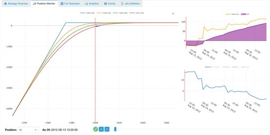
QuantPedia Composite ShortPut RiskGraph

Backtest run is available here: 
https://mesosim.deltaray.io/backtests/229fe2c8-483c-4ab4-b8e4-403df2b7e6ed

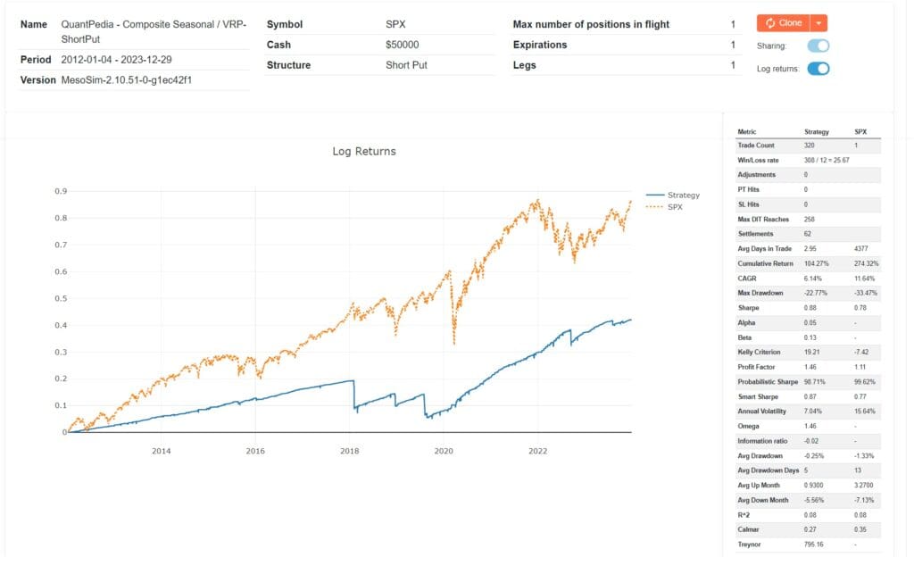
QuantPedia Composite ShortPut Overview

The results show that volatility risk premium harvesting combined with market timing can be a highly profitable majority of the time, but the infrequent losses can wipe multiplied days of profits. The losses experienced during the above run were linked to significant market downturns, including the dramatic stock market events of 2018: Volmageddon and the worst U.S. stock decline since 2008, as well as the 2019 downturn driven by the US-China trade war.

In the next step, we will address the infrequent losses using an options-specific stop-loss mechanism.

Step 3: VRP – Short Put with StopLoss

Controlling for risk is essential in all trading strategies. There are several methods to minimize downside risk in options-based strategies. You can decide to exit or adjust a position based on:

• Option moneyness, for example, when the underlying price falls below the strike price.
• Position Delta, for example, if the delta exceeds 50.
• The comparison of Profit and Loss against the Credit Received.
• Other factors include implied volatility (IV), other Greeks like theta, and market volatility indices such as VIX or VVIX.

We will focus on exploring the first three methods in detail.

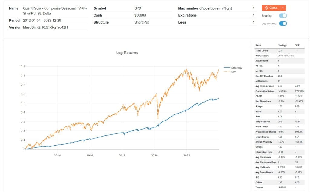
Option moneyness based

When the underlying price drops below the option’s strike price, e.g. when the Short Put contract becomes In The Money (ITM) the rate-of-loss of the position accelerates. It is therefore logical to exit a position at the point (or before) when the strike is breached. In MesoSim this can be defined as:
“Exit”: {
     “Conditions”: [
           “underlying_price < leg_short_put_strike”
     ],
     …
  }

Backtest run can be viewed here:
https://mesosim.deltaray.io/backtests/26eb380b-abb4-48d1-91bd-2f16d3282c53

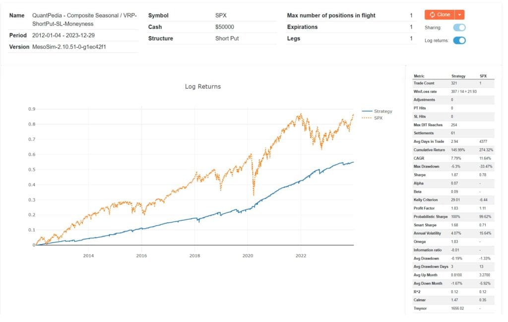
QuantPedia Composite ShortPut SL Moneyness overview

Delta based

Delta values around 50 typically indicate that an options is somewhere around At The Money (ATM). However, it’s important to note that an option may not always exactly match a delta of 50 when it is ATM due to varying market conditions and specific characteristics of the option. As the delta exceeds 50, the option moves further into-the-money (ITM). To manage risk effectively and to exit a position when it’s delta becomes larger than 50, you can use the following Exit Condition in MesoSim:

“Exit”: {
     “Conditions”: [
           “pos_delta > 50”
     ],
 }

For further insights, please refer to our backtest run, accessible: https://mesosim.deltaray.io/backtests/38cc3635-cb09-4cca-b3ee-89a247ed0305

QuantPedia Compose ShortPut SL Delta overview

Note that the curve is matching the Moneyness based run as the Delta selection is matching the deltas of ATM options.

Credit received based

In short-dated option selling strategies the StopLoss is often described as a function of credit received. You might decide to exit a position if losses exceed a predetermined multiple of the initial credit. To have a 2:1 Risk/Reward ratio we can trigger a sell by using the Option Premium for the put we sold.

First we need to capture the Option Price on entry:
“Entry”: {
     “VarDefines”: {
           …
           “credit_received”: “leg_short_put_price * abs(leg_short_put_qty) * 100”
     },
     …
}

Then, we use the credit_received variable to exit when the position PnL reaches 2 times of the value:
“Exit”: {
    “Conditions”: [
     “pos_pnl < (-1 * 2 * credit_received)”
     ],
     …
}

For detailed performance metrics, please refer to our backtest run: https://mesosim.deltaray.io/backtests/c395cb1a-7010-47b4-ae62-4796fbd51619

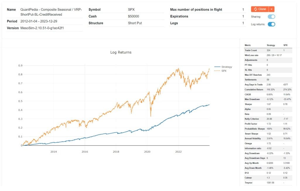
QuantPedia Composite ShortPut SL CreditReceived overview 

The final step involves applying position sizing.

Step 4: VRP Sizing

The above runs used a fixed, initial account size of $50,000 for the trade. That account size was chosen so that the positions can be entered using a Reg-T account. Options are often traded using Portfolio Margin or SPAN based margin accounts, which allow for greater leverage. At the time of writing, a 10 delta Short Put on SPX requires $12,000 of buying power for 1 Day to Expiration (DTE) and $9,000 for 5 DTE. Adopting a conservative strategy, we use only 50% of our buying power, scaling down the initial cash to $25k for the StopLoss based trades.

The efficacy of this approach is evident when compared against the SPX, where it achieves a comparable performance, but with lower drawdown of 8.26% (versus 33.47%) and a more favorable Sharpe ratio of 1.98 (compared to 0.77). Importantly, this strategy is active in the market only 40% of the time, demonstrating its efficiency by limiting market exposure while still capturing significant returns.

For detailed performance metrics and further insights, please refer to our recent backtest run, accessible: https://mesosim.deltaray.io/backtests/460a6563-e35d-4296-9a83-a8f200737c84

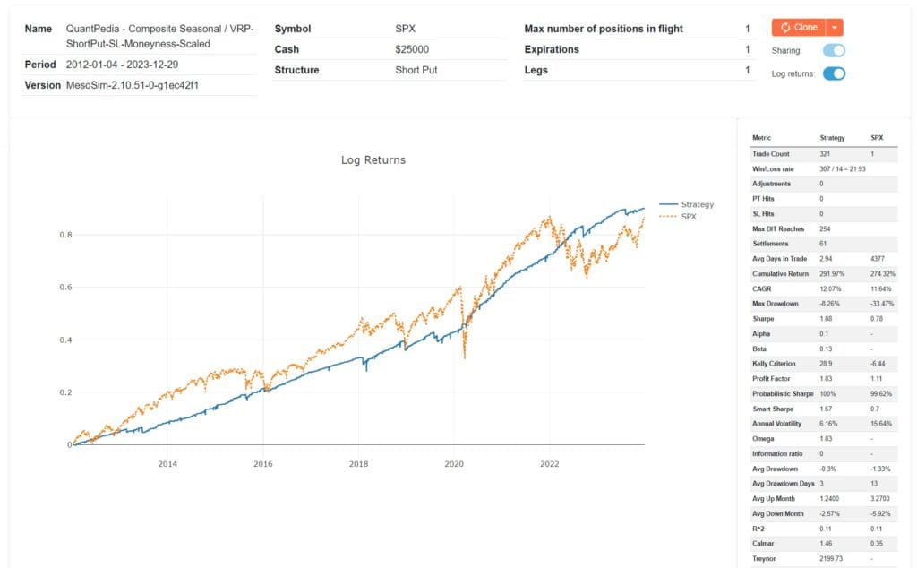
QuantPedia Composite ShortPut SL Moneyness Scaled

Conclusion

In collaboration with Deltaray, we applied Quantpedia’s Composite Seasonal/Calendar Strategy to options trading, gaining valuable insights into how seasonal anomalies can be used in the options market. Our main goal was to not only replicate QuantPedia’s findings but also to enhance them by effectively using the Volatility Risk Premium (VRP).

Initially, we prepared our data by marking critical market indicators such as option expirations and FOMC meeting dates. We then used MesoSim to simulate stock holdings through synthetic long positions. After establishing a solid baseline, we examined the advantages of VRP with a Short Put strategy, discovering that although it often leads to significant profits, it also comes with the risk of severe losses. To mitigate these risks, we applied StopLoss mechanisms based on delta values, option moneyness, and credit received, which significantly improved our risk management.

Our final approach involved using the Short Put strategy and a conservative position sizing to optimize trading conditions. This improved our Sharpe ratio and Drawdown metric when compared to SPX.

Future work will refine our strategies further through sensitivity analyses and by adding hedging component, specifically long puts.

---

Deltaray’s MesoSim is an options strategy simulator with unique flexibility and performance. You can create, backtest, and optimize options and trading strategies on equity indexes and crypto options at a lightning-fast speed. Now, it’s integrated with ChatGPT to assist users in creating backtest job definitions.

Exclusively, only for the Quantpedia community, our readers can now use the coupon code QUANTJUNE to obtain a 30% discount on new annual subscriptions for both the Standard and Advanced Plans. The coupon is valid between 13th June and 20th June 2024.

---

Are you looking for more strategies to read about? Sign up for our newsletter or visit our Blog or Screener.

Do you want to learn more about Quantpedia Premium service? Check how Quantpedia works, our mission and Premium pricing offer.

Do you want to learn more about Quantpedia Pro service? Check its description, watch videos, review reporting capabilities and visit our pricing offer.

Are you looking for historical data or backtesting platforms? Check our list of Algo Trading Discounts.

Do you have an idea for systematic/quantitative trading or investment strategy? Then join Quantpedia Awards 2024!

---

Or follow us on:

Facebook Group, Facebook Page, Twitter, Linkedin, Medium or Youtube

---

References

[1] ALMUDHAF, Fahad. The Islamic calendar effects: Evidence from twelve stock markets. Available at SSRN 2131202, 2012.

[2] ARIEL, Robert A. A monthly effect in stock returns. Journal of financial economics, 1987, 18.1: 161-174.

[3] EHRMANN, Michael; JANSEN, David-Jan. The pitch rather than the pit: investor inattention during FIFA World Cup matches. 2012.

[4] Ma, Aixin and Pratt, William Robert, Payday Anomaly (September 28, 2018). Available at SSRN: https://ssrn.com/abstract=3257064  or http://dx.doi.org/10.2139/ssrn.3257064

[5] MesoSim portal by Deltaray. MesoSim Portal by deltaray. (n.d.). Available at: https://mesosim.deltaray.io/

[6] OSBORNE, Maury FM. Periodic structure in the Brownian motion of stock prices. Operations Research, 1962, 10.3: 345-379.

[7] ROZEFF, Michael S.; KINNEY JR, William R. Capital market seasonality: The case of stock returns. Journal of financial economics, 1976, 3.4: 379-402.

[8] Stivers, C., & Sun, L. (2013). Returns and option activity over the option-expiration week for S&P 100 stocks. Journal of Banking & Finance, 37(11), 4226-4240.

[9] Tori, C. R. (2001). Federal Open Market Committee meetings and stock market performance. Financial Services Review, 10(1-4), 163-171.

[10] U.S. Federal Reserve (FED) meeting minutes. (n.d.). Investing.com. Available at: https://www.investing.com/economic-calendar/fomc-meeting-minutes-108

[11] Vojtko, R., & Padyšák, M. (2019, April 26). Case study: Quantpedia’s composite seasonal / calendar strategy. QuantPedia. Available at: https://quantpedia.com/quantpedias-composite-seasonalcalendar-strategy-case-study/

Share onLinkedInTwitterFacebookRefer to a friend