The Active vs Passive: Smart Factors, Market Portfolio or Both?
We would like to present our newest own-research about factor allocation and passive versus active strategies clash. However, respecting our blog format, this version is largely shortened and we invite you to read the full version.
Introduction
In the equity market, there are two types of investing: active and passive. The aim of passive investors is to track the market with all the “ups” and “downs”. The passive investing is simple; after all, the strategy consists of tracking the market by a buy-and-hold. Nowadays, it is easy to implement with the numerous ETFs, for example, by buying SPY ETF and getting exposure to the S&P500 index. Proponents state that in the long run, the equity market is going up. They do not try to beat the market, they bet on the market in the long run.
On the other hand, there is active management. The main aim of active investing should be to beat the market. Therefore, active investors aim to achieve better returns or risk-adjusted returns since the equity markets tend to be volatile. The passive investors should aim for a long horizon, and therefore, they should not panic when they experience the first drawdown. However, for many, it is desired that their investment would be more stable or safe. A major part of active investment management consists of factor (or smart beta) strategies. Equity factors include, for example, value, size, volatility, momentum or quality. With the numerous ETFs, it is also easy to get exposure to these factors through smart beta ETFs.
Is active or passive investing better?
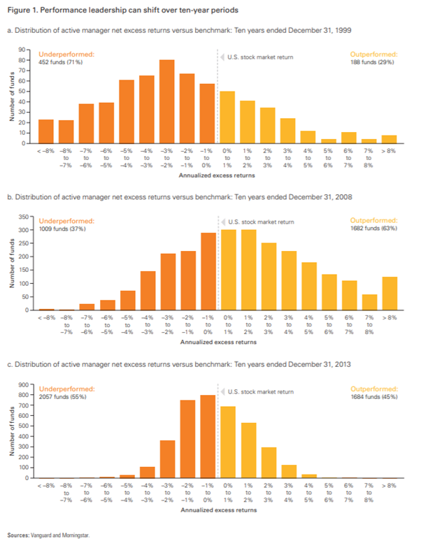
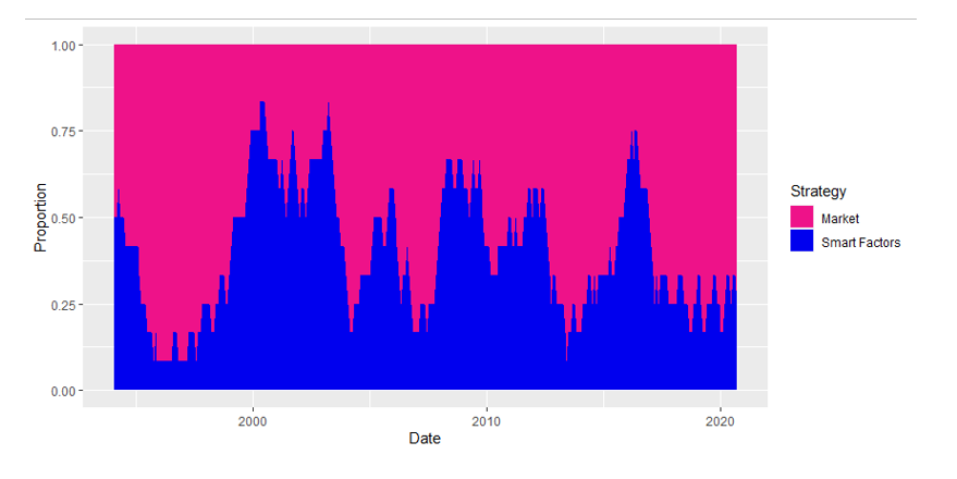
Having established that there are two major management styles and many factors, numerous questions arise. Firstly, there is a debate that is as old as investing itself, is active or passive investing better? There seems to be an unreasonable debate, many investing “experts” shame active investing stating that active managers often cannot beat the market. Indeed, the active management requires skill and knowledge, which can bring success, and outperform the market (either in total or risk-adjusted returns). On the other hand, passive management does not require much of the skill or knowledge and with low-cost brokers, and ETFs, it is widely accessible to retail investors. The truth lies somewhere in the middle. The performance of active and passive investing is cyclical. The periods of active (passive) outperformance rotate (see the following figure). Therefore, the answer to the question of which investing is better, changes in time. We should find a solution to a different problem, in which state of the market is it better to invest passively and in which state of the market is it better to invest actively? Another question that arises is whether we can use our active investing strategy to outperform the market consistently.
| Algo Trading Data Discounts are available exclusively for Quantpedia’s readers. |
Considering active investing, if we get back to the factor investing, we have a similar ongoing debate. It is widely recognized that equity factors also have cyclical performance. Many argue that value is dead (which has already happened in the past), yet Blitz and Hanauer (2020) claim that value can be resurrected. Momentum is notoriously known for its crashes (Hanauer and Windmüller, 2020). Also, the size factor seems to have its problems (Blitz and Hanauer, 2020). On the other hand, quality appears to be emerging as a popular investment style, and it has even enjoyed outperformance compared to the other factor during the recent first Covid wave (Quantpedia, 2020).
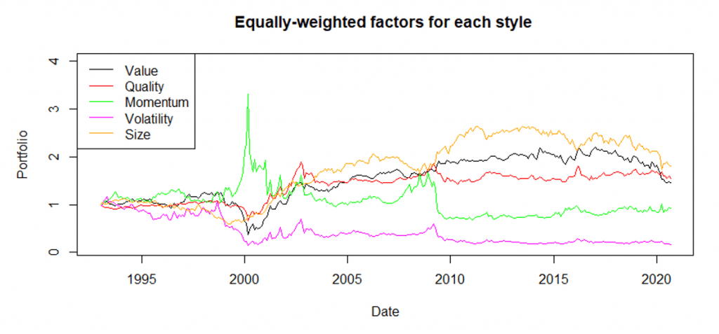
Establishing that factor investing is not that straightforward and has cyclical performance, the aim of this paper is to find a profitable way how to invest in plenty of equity factors. Factors are obtained from the Alpha Architect’s Factor Investing Data Library. The factor library includes all the major styles: Value, Momentum, Volatility, Quality and Size. We are interested in two markets: the US market that is represented by the top 1500 stocks and developed market (EAFE). Through the paper, the analysis is made for both markets.
Achilles’ heel of time-series momentum portfolios
Since the performance of the factors is cyclical, the hypothesis of the paper is that each factor could be a vital part of the final portfolio. However, the weight of each factor in the portfolio should be changing in time. A possible way is to react to the actual market situation. Garg et al. (2019) examined the time-series momentum strategies and the momentum turning points. According to the research, turning points are the Achilles’ heel of time-series momentum portfolios. The reason is straightforward, slow signals tend to be unreactive to changes in trend, and fast signals are often false alarms. The authors examine fast and slow momentum signals and different blending approaches to construct more profitable momentum strategies. The weight of the long (short) position depends on both fast and slow signals, and whether they agree or disagree. We follow a similar approach for the construction of the factor momentum strategies, but there are major differences. For the active factor strategy, we first examine two signals: fast, which is 1-month momentum and slow, which is 12-month momentum. Moreover, we examine the strategy which is traded only if both signals agree and blended strategy similar to the Garg et al. (2019).
Nextly, separately for each type of signal and for each factor, we cross-sectionally rank the absolute value of the signal to obtain the strength of the signal. The ranks act like weights – stronger the signal greater the weight. After establishing cross-sectional strength, the factor strategies that utilize the slow and fast signals can be further enhanced. The detailed strategies and results can be found in the sections 3, 4 and 5 in the paper.
Dynamic weighting
The dynamic weighting outperforms the baseline strategies. The outperformance of dynamical weighting compared to all other strategies is present on each market and each type of portfolio sort (quintiles, deciles and ventiles). Moreover, the results of the dynamic weighting of signals outperform other strategies in two distinct approaches. Firstly, when we consider the relative strength of the signals for all factors together or in the other case, when we firstly, break all the factors into individual investment styles separately. The results are almost exactly the same (since the breaking the factors into individual styles does not alter the results, for the simplicity, results for such variant are unpublished).
It is worth mentioning that by the construction, all of the strategies are “immune” to problems like value versus growth or short-term momentum/short-term reversal. For example, if the value tends to be profitable, the strategy would tilt its exposition to the value factors. If the value tends to be unprofitable (growth is profitable), the strategy shorts the value factors (in other words, it reverses deciles, quintiles or any other sorted portfolios).
Active versus passive investing
Having established that it is possible to utilize the factors better in a relative-strength dynamically weighted factor momentum strategies, it is time to get back to the active versus passive investing debate. In the recent period, it is well-known that many factors have underperformed.
Therefore, it seems that in the past, proponents of passive investing were right. However, that conclusion would not be correct. Later, we show that active investing, using the relative-strength dynamically blended factor momentum strategy could be a great addition to the market portfolio. The combined strategy looks back on the past twelve months, and twelve moving averages (MA) of the returns: one month, two months, three months and so on. Suppose the MA for active investing (factor momentum) is larger than MA for market portfolio, then the active investing scores one point. Otherwise, the market portfolio gets one point. Therefore, each month, the weight of the factor momentum and market portfolio is determined by the number of “winning” (loosing) moving averages. Combining active and passive investing largely outperforms passive investing only. Moreover, if we have a rule that we follow for investing into factors and market, it is definitely an active investing strategy.
Although the relative-strength dynamically blended factor momentum strategy and its combination with the market portfolio might seem to be tangled, the rules are straightforward and transparent. It is possible to ex-post choose the best lookback periods for fast and slow indicators, or the best blending rule, however, such overfitting is not in the interest of this paper. Strategies should be transparent, and the aim of this paper is to show a set of transparent rules to find answers to two questions. Firstly, which factor to invest in (factor allocation problem), and secondly, to have a rule-based solution to the active versus passive clash.
Data
Factors are obtained from the Alpha Architect’s Factor Investing Data Library. The factors include Asset Growth, Beta, Book/Price, Cash Flow/Price, Debt Paydown Yield, Dividend/Price, Earnings/Price, EBIT/TEV, EBITDA/TEV, Financial Strength Score, Gross Profit, various Momentum measures (1m, 6m, 12m and 12m with the last month skipped), Repurchase Yield, Return on Assets, Return on Equity, Sales/Price, Shareholder Yield, Shareholder Yield with Debt, Size and Volatility. Therefore, the factor library includes all the major styles: Value, Momentum, Volatility, Quality and Size.
All factors are either value-weighted or equally-weighted. We are interested in two markets: the US market that is represented by the top 1500 stocks and developed market (EAFE). The data spans from 31.1.1993 to 31.8.2020, therefore, it includes many major financial crises, e.g. the dot-com bubble, the financial crisis of 2007–2008, recent COVID crisis (the first wave, including the recovery) and many other market downturns.
Methodology
This section is largely shortened and includes only the main principles. Detailed approach and equations are in the original paper.
We are interested in two signals: fast, which is 1-month momentum and slow, which is 12-month momentum. Moreover, we examine the strategy which is traded only if both signals agree and blended strategy. The blended strategy reduces exposure to the factors if the fast and slow signals disagree. If the fast signal is already positive, but the slow is still negative, the factor has a reduced long position to one half. If the slow signal is still positive, but the fast is negative, there is a reduced short position to one half.
Additionally, we recognize the “dynamic” strategies, where separately for each type of signal and each factor, we cross-sectionally rank the absolute value of the signal to obtain the strength of the signal. The ranks act like weights – stronger the signal greater the weight.
The combination of active factor strategy and market portfolio is straightforward, the combined strategy looks back on the past twelve months, and twelve MAs of the returns. If the MA for active investing (factor momentum) is larger than MA for market portfolio, the active investing scores one point. Otherwise, the market portfolio gets one point. Therefore, each month, the weight of the factor momentum and market portfolio is determined by the number of “winning” (loosing) moving averages.
Results – US Stocks
| Strategy | Return | Volatility | Max Drawdown | Risk-adjusted performance |
| Slow | 3.362% | 10.969% | -38.075% | 0.306 |
| Fast | 3.235% | 11.032% | -24.445% | 0.293 |
| Neutral | 3.547% | 8.464% | -22.83806 | 0.419 |
| Dynamically neutral | 4.402% | 11.224% | -27.783% | 0.392 |
| Blended | 3.451% | 9.183% | -20.911% | 0.376 |
| Dynamically blended | 4.235% | 12.133% | -26.303% | 0.349 |
Table 1 Performance metrics for strategies mentioned in section 3 in the US market. Returns and volatilities are annualized. Risk-adjusted performance is return divided by the volatility. The sample consists of returns for the period of 31.12.1992 to 31.8.2020. Individually, each factor is value-weighted. The factor portfolios are weighted according to section 3. The Slow is the long term momentum signal (12 months), Fast signal is the short term momentum signal (1 month), Neutral trades only if both signals agree, Blended strategy reduces the weight in the times when the slow and fast indicator do not agree (equation 11). Dynamic strategies employ relative weights (the strength of each signal – equations 3 and 4).
The dynamical approach improves the performance of both neutral and blended strategies. However, by the construction, both strategies are blended with different weights for short and fast signals. As expected, dynamical strategies are the most profitable. The blending of the signals adds some performance (measured by the returns) compared to slow or fast signals. Therefore, the blending of time-series factor momentum signals seems to be profitable. Even larger returns were obtained with dynamic strategies that are similar to the cross-sectional momentum.
The performance can also be inspected visually, by looking at the equity lines for the unit portfolios.
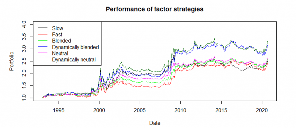
All of the strategies are profitable, do not have large drawdowns or volatilities, but they do not seem to be that profitable. There are many periods where the performance is flat.
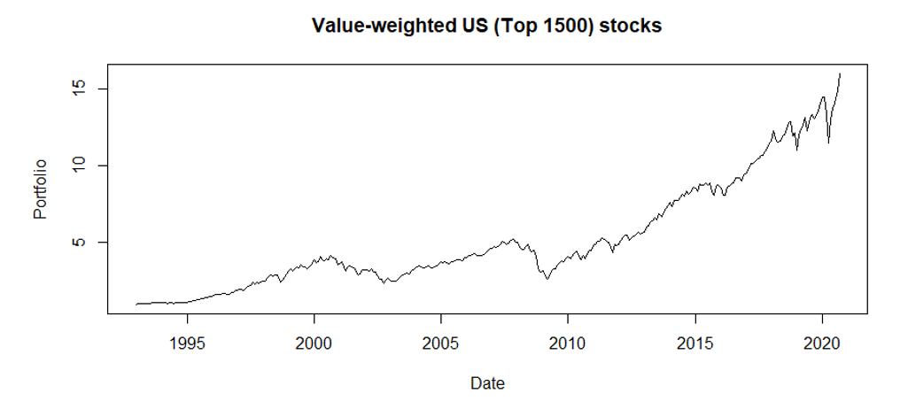
Compared to the factor strategies, a buy-and-hold approach for top 1500 US stocks would have skyrocketed. A natural question arises, is there any reason to invest in factors?
Common knowledge is that the outperformance of active and passive investing is cyclical. The edge is changing based on market conditions. Therefore, we suggest that both the active factor strategy and market portfolio should be utilized in the investor’s portfolio. However, there needs to be set a rule for the allocations. This common-sense can also be backed by the correlations between active and passive strategies. Spearman’s correlation coefficient between the market portfolio and dynamically blended strategy is -0.185 (p-val 0.0006969). Coefficient between dynamically neutral strategy and market portfolio is -0.143 (p-val 0.009194). Both correlations are negative and highly statistically significant using non-parametric (therefore robust in this case) tests. These results suggest that it should be beneficial to combine those strategies. The performance of active and passive investing is cyclical and slightly negatively correlated. The straightforward rules based on simple moving averages were established in section 4. Throughout the next section, the combination is presented for the market portfolio and dynamically blended strategy that would be called the Smart Factors.
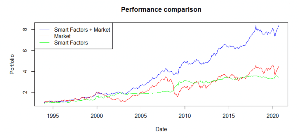
| Strategy | Return | Volatility | Max Drawdown | Risk-adjusted performance |
| Smart Factors | 3.884% | 12.282% | -26.303% | 0.316 |
| Market | 10.519% | 15.086% | -50.007% | 0.697 |
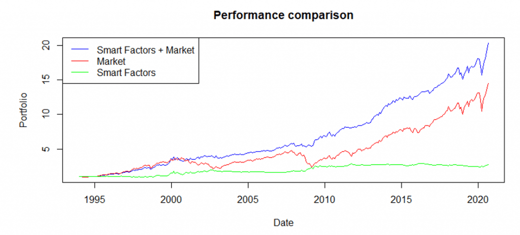
| Smart Factors + Market | 11.909% | 10.460% | -16.95% | 1.138 |
The combination of Smart Factors + market demonstrates the potential of the factor strategies. Gathering information from Figure 1-3, factors are profitable when the market is not, and by the construction (section 4), the combination strategy has the biggest allocation into factors when there is a market downturn. On the other hand, the factors tend to be flat when the market is largely profitable. As a result, the combination has the largest return, the lowest volatility and max drawdown, and the highest risk-adjusted-performance. A dollar invested in the 31.12.1993 would result in the 20.28 dollars by the 31.8.2020 compared to only 14.52 dollars for the Market portfolio.
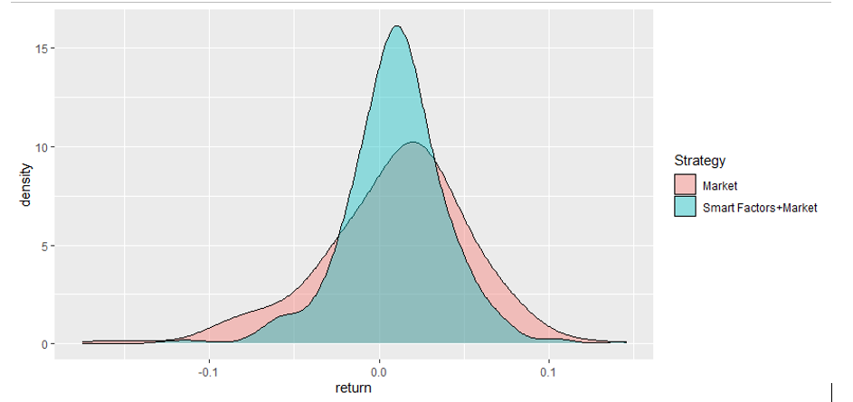
Returns of the combination strategy also tend to be more favourably distributed. The left tail is shorter and thin, not as heavy as for market portfolio. As expected, the same can be said about the right tail, but overall, the combination is better.
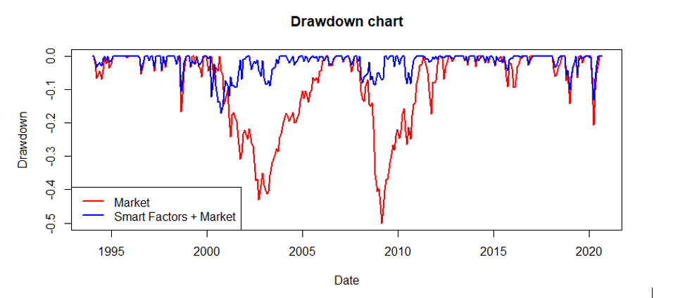
The list of favourable properties does not end; the following chart shows the much lower drawdowns for the combined portfolio. While one could say that the passive approach is better than some factor (smart beta) strategies, and passive investing is superior to the active, their active combination and dynamic allocation largely outperforms the passive buy-and-hold approach of the market.
Results – EAFE Stocks
The same analysis is also available for the EAFE stocks, but in the blog post, we only include the main result: comparison of Smart Factors, Market and Smart Factors + Market.
Conclusion
We conclude that the results are qualitatively the same for both investments universes. In both EAFE and US stocks, the market portfolio in terms of returns outperforms the factor strategies. The results hold even if we use time-series, cross-sectional factor momentum or blending the fast and slow momentum signals. However, the blending of the fast and slow signals proved to be superior to using the fast or slow signals only. Overall, the results are in line with the known results for momentum anomalies in the individual stocks.
It might look like that the passive approach of buy-and-hold market indices outperforms the active investing, and the active investing is pointless, but we show that this simply is not true. The active approach that consists of smart allocation into both Smart Factors strategy and market portfolio significantly outperforms either market or factors. Smart Factors and market are in both cases, slightly negatively correlated. The performance of both is cyclical, and factors have an outstanding performance during market downturns. Therefore, by allocating into market and factors using a scoring system based on moving averages, it is possible to create much more profitable portfolio, with lower volatility or drawdowns. These results are applicable to both markets – US and EAFE. In both cases, the risk-adjusted return dramatically improves switching from market portfolio to the combined portfolio (from 0.361 to 0.995 for EAFE stocks and from 0.697 to 1.138 for US stocks). Lastly, comparing the factors and markets, the EAFE factors outperform US factors, but US market outperforms the EAFE market. Therefore, the combined portfolio in the connected samples could be an interesting idea for a further research.
Author:
Matus Padysak, Senior Quant Analyst, Quantpedia
Related literature
[1] Arnott, Robert D. and Clements, Mark and Kalesnik, Vitali and Linnainmaa, Juhani T., Factor Momentum (February 1, 2019). Available at SSRN: https://ssrn.com/abstract=3116974 or http://dx.doi.org/10.2139/ssrn.3116974
[2] Blitz, David and Hanauer, Matthias Xaver, Resurrecting the Value Premium (October 15, 2020). Available at SSRN: https://ssrn.com/abstract=3705218 or http://dx.doi.org/10.2139/ssrn.3705218
[3] Blitz, David and Hanauer, Matthias Xaver, Settling the Size Matter (September 4, 2020). Available at SSRN: https://ssrn.com/abstract=3686583 or http://dx.doi.org/10.2139/ssrn.3686583
[4] Christopher B. Philips, CFA; Francis M. Kinniry Jr., CFA; David J. Walker, CFA: The Active-Passive Debate: Market Cyclicality and Leadership Volatility (July 2014). Vanguard research. Available at: https://personal.vanguard.com/pdf/ISGACT.pdf
[5] Garg, Ashish and Goulding, Christian L. and Harvey, Campbell R. and Mazzoleni, Michele, Momentum Turning Points (December 9, 2019). Available at SSRN: https://ssrn.com/abstract=3489539 or http://dx.doi.org/10.2139/ssrn.3489539
[6] Gupta, Tarun and Kelly, Bryan T., Factor Momentum Everywhere (November 1, 2018). Yale ICF Working Paper No. 2018-23, Available at SSRN: https://ssrn.com/abstract=3300728 or http://dx.doi.org/10.2139/ssrn.3300728
[7] Hanauer, Matthias Xaver and Windmüller, Steffen, Enhanced Momentum Strategies (August 07, 2020). Available at SSRN: https://ssrn.com/abstract=3437919 or http://dx.doi.org/10.2139/ssrn.3437919
[8] Quantpedia: YTD Performance of Equity Factors – Update After Two Months (15.May 2020). Quantpedia’s blog. Available at: https://quantpedia.com/ytd-performance-of-equity-factors-update-after-two-months/
Are you looking for strategies applicable in bear markets? Check Quantpedia’s Bear Market Strategies
Are you looking for more strategies to read about? Sign up for our newsletter or visit our Blog or Screener.
Do you want to learn more about Quantpedia Premium service? Check how Quantpedia works, our mission and Premium pricing offer.
Do you want to learn more about Quantpedia Pro service? Check its description, watch videos, review reporting capabilities and visit our pricing offer.
Do you want algorithmic access to the full Quantpedia database via the API? Subscribe to Quantpedia Pro, ask for an API key, and explore the in/out-of-sample statistics, source academic papers, and code snippets — ideal for quantitative research, systematic trading workflows, and AI model training.
Are you looking for historical data or backtesting platforms? Check our list of Algo Trading Discounts.
Or follow us on:
Facebook Group, Facebook Page, Telegram, Twitter, Linkedin, Medium or Youtube
Share onLinkedInTwitterFacebookRefer to a friend


